Site Energy Usage Intensity Prediction
Energy usage intensity (EUI) refers to the amount of energy used per square foot annually. It is calculated by dividing the total energy consumed by the building in a year by the total gross floor area. Like miles per gallon for cars, EUI is the prime indicator of the energy performance of a building. In this project, we aim to predict the continuous target variable site EUI, given the characteristics of the building and the weather data for its location.
○ Contents
- Overview
- Introduction
- Exploratory Data Analysis
- Data Preprocessing
- Feature Engineering
- Baseline Modeling
- Hyperparameter Tuning
- Prediction and Evaluation
- Acknowledgements
- References
○ Overview
- Energy usage intensity (EUI) refers to the amount of energy used per square foot annually. It is calculated by dividing the total energy consumed by the building in a year by the total gross floor area. Like miles per gallon for cars, EUI is the prime indicator of the energy performance of a building.
- The EUI of a site or a building may depend on
- building characteristics: floor area, facility type etc.
- weather data for the location of the building: annual average temperature, annual total precipitation etc.
- In this project, we aim to predict the continuous variable site EUI, given the characteristics of the building and the weather data for the location of the building.
- A detailed exploratory data analysis on the dataset is carried out.
- The observations obtained from EDA are used in the data preprocessing stages (consisting of missing data imputation and categorical data encoding) and feature engineering stages (consisting of feature extraction, data transformation, and binarization).
- We employ the random forest, XGBoost, and CatBoost regressors to predict site EUI.
- We apply hyperparameter tuning to the random forest algorithm, which appears to perform best among the baseline candidates.
- We employ the root mean square error (RMSE), mean absolute error (MAE), and coefficient of determination (\(R^2\)) metrics to evaluate the models. Performance summary of the final model:

○ Introduction
Data
The dataset contains roughly \(100\) thousand observations of building energy usage records collected over \(7\) years, in several states within the United States. It consists of building characteristics (e.g. floor area, facility type etc.), weather data for the corresponding location of the building (e.g. annual average temperature, annual total precipitation etc.) as well as the energy usage for the building in the given year, measured as Site Energy Usage Intensity (Site EUI). Each row in the data corresponds to a single building observed in a given year.
A snapshot of the training set:

A snapshot of the test set:

Project Objective
The objective of the project is to predict energy usage intensity of a building in a given year, based on building characteristics as well as weather data for the location of the building.
Evaluation Metric
The true values of the target variable, which is the Site EUI, is provided in the test dataset. We use the trained models to predict this variable for each row of the test dataset and evaluate the models in terms of the root mean square error. Apart from this metric, we also report mean absolute error (MAE) and coefficient of determination (\(R^2\)) for model evaluation.
○ Exploratory Data Analysis
Understanding Features
- year_factor: anonymized year in which the weather and energy usage factors were observed
- state_factor: anonymized state in which the building is located
- building_class: building classification
- facility_type: building usage type
- floor_area: floor area (in square feet) of the building
- year_built: year in which the building was constructed
- energy_star_rating: the energy star rating of the building
- elevation: elevation of the building location
- january_min_temp: minimum temperature in January (in Fahrenheit) at the location of the building
- january_avg_temp: average temperature in January (in Fahrenheit) at the location of the building
- january_max_temp: maximum temperature in January (in Fahrenheit) at the location of the building
(Similarly for all other months)
- cooling_degree_days: cooling degree day for a given day is the number of degrees where the daily average temperature exceeds 65 degrees Fahrenheit. Each month is summed to produce an annual total at the location of the building.
- heating_degree_days: heating degree day for a given day is the number of degrees where the daily average temperature falls under 65 degrees Fahrenheit. Each month is summed to produce an annual total at the location of the building.
- precipitation_inches: annual precipitation in inches at the location of the building
- snowfall_inches: annual snowfall in inches at the location of the building
- snowdepth_inches: annual snow depth in inches at the location of the building
- avg_temp: average temperature over a year at the location of the building
- days_below_30F: total number of days below \(30\) degrees Fahrenheit at the location of the building
- days_below_20F: total number of days below \(20\) degrees Fahrenheit at the location of the building
- days_below_10F: total number of days below \(10\) degrees Fahrenheit at the location of the building
- days_below_0F: total number of days below \(0\) degrees Fahrenheit at the location of the building
- days_above_80F: total number of days above \(80\) degrees Fahrenheit at the location of the building
- days_above_90F: total number of days above \(90\) degrees Fahrenheit at the location of the building
- days_above_100F: total number of days above \(100\) degrees Fahrenheit at the location of the building
- days_above_110F: total number of days above \(110\) degrees Fahrenheit at the location of the building
- direction_max_wind_speed: wind direction for maximum wind speed at the location of the building. Given in \(360\)-degree compass point directions (e.g. \(360\) = north, \(180\) = south, etc.).
- direction_peak_wind_speed: wind direction for peak wind gust speed at the location of the building. Given in 360-degree compass point directions (e.g. \(360\) = north, \(180\) = south, etc.).
- max_wind_speed: maximum wind speed at the location of the building
- days_with_fog: number of days with fog at the location of the building
- building_id: building id
- site_eui (target variable): Site Energy Usage Intensity is the amount of heat and electricity consumed by a building as reflected in utility bills
Data Synopsis
Training data synopsis
- Number of observations: \(85462\)
- Number of columns: \(64\)
- Number of integer columns: \(37\)
- Number of float columns: \(24\)
- Number of object columns: \(3\)
- Number of duplicate observations: \(0\)
- Constant columns: None
- Number of columns with missing values: \(6\)
- Columns with missing values:
year_built,energy_star_rating,direction_max_wind_speed,direction_peak_wind_speed,max_wind_speed,days_with_fog - Memory Usage: \(37.57\) MB
Test data synopsis
- Number of observations: \(9705\)
- Number of columns: \(64\)
- Number of integer columns: \(37\)
- Number of float columns: \(24\)
- Number of object columns: \(3\)
- Number of duplicate observations: \(0\)
- Constant columns:
year_factor,days_above_110F - Number of columns with missing values: \(6\)
- Columns with missing values:
year_built,energy_star_rating,direction_max_wind_speed,direction_peak_wind_speed,max_wind_speed,days_with_fog - Memory Usage: \(4.74\) MB
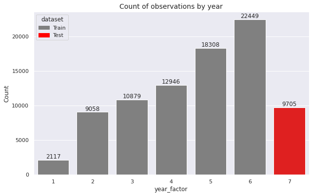
We observe that the training set contains information for six years (year_factor = \(1\)
to year_factor = \(6\))
and the test set contains information for the seventh year (year_factor = \(7\)).
Univariate Analysis
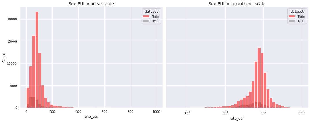
We begin with the target variable site_eui, which is a continuous variable indicating the amount of heat and electricity consumed by a building as reflected in utility bills.
Observations
- The distribution of
site_euiis positively skewed - On the logarithmic scale it approaches a bell-shaped distribution
Next, we consider the predictor variables. First, we identify the almost constant columns.
- The feature
days_above_110Fis almost constant in the sense that it is \(0\) for \(99.91\%\) of the training observations and for \(100\%\) of the test observations - The feature
days_above_100Ftakes the value \(0\) for \(94.63\%\) of the training data and for \(89.41\%\) of the test data
Now we detect the columns with unrealistic values as majority.
- The feature
direction_max_wind_speedis \(1.0\) for \(79.95\%\) of the training observations - The feature
direction_peak_wind_speedis \(1.0\) for \(81.59\%\) of the training observations - The feature
max_wind_speedis \(1.0\) for \(79.95\%\) of the training observations
In all the three columns for both training data and test data \(1.0\) is an extremely isolated point.
Also, we observe that there are \(6\)
observations in the training data and \(1\)
observation in the test data which were apparently built in the year \(0\).
These are probably incorrect because the year \(0\)
is an extremely rare point in the year_built column for both the training data and the test data. We keep a copy of the data with these unrealistic \(0\)-values
in the year_built column to NaN.
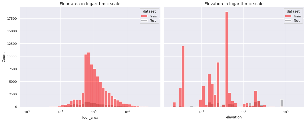
Next, we present the histograms of the numerical features in the data except the almost constant column days_above_110F, the columns with unrealistic values as majority direction_max_wind_speed, direction_peak_wind_speed, max_wind_speed, and the columns year_factor and building_id.

Observations
floor_areaandelevationhave positive skewness to an extreme degreeenergy_star_ratingis negatively skewed to a moderate degree- The oldest building in the dataset was built in the year \(1600\)
- The latest building in the dataset was built in the year \(2016\)
- Most buildings in both the training data and the test data were built after the year \(1900\)
- A massive number of buildings were built during the second half of \(1920\)'s and the beginning of \(1960\)'s
- The sudden drops in the count during the two world wars \((1914-1918\) and \(1939-1945)\) are clearly noticeable
We apply the logarithmic scale on extremely skewed distributions.
Next, we compare the frequency of observations by year.
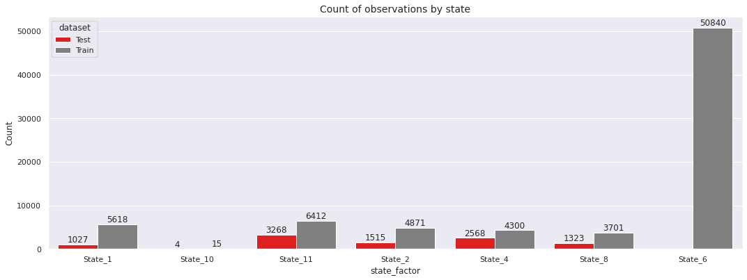
We follow this us with a frequency comparison by state.
Observations
- Majority of the training data comes from
State_6 - The test data has no observation from
State_6
The building_class can be either commercial or residential. We compare the frequencies for these two categories.
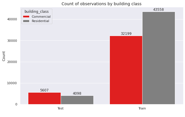
Observations
- The training data contains more
residentialbuildings - The test data contains more
commercialbuildings
Next, we present a relational plot to show the frequency comparison of different types of facilities.
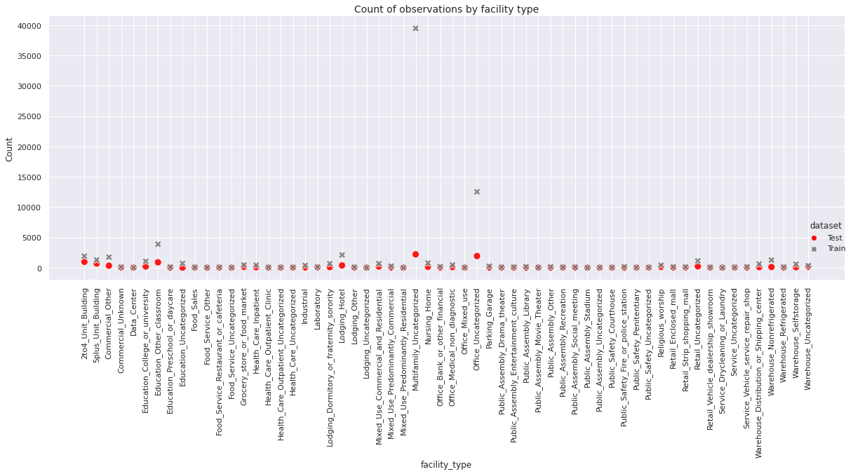
There are several object type variables, for which certain values appear only rarely in the dataset. For visualization purpose, we merge these rarely occurring values into the label Others, in a copy of the dataset.
The following function takes a column col of a DataFrame data, detects its values with relative frequency less than a certain cutoff with the default value set at \(0.01\),
and replace those values by the label Others. The function is useful in incorporating the merging operation in the visualization of frequency comparison of object type variables that take a lot of values.
def merge_val(data, col, cutoff = 0.01):
    data_temp = data.copy(deep = True)
    val_major_list = data[col].value_counts()[data[col].value_counts()/len(data) >= cutoff].index.tolist()
    val_minor_list = data[col].value_counts()[data[col].value_counts()/len(data) < cutoff].index.tolist()
    val_dict = {}
    for val in val_major_list:
        val_dict[val] = val
    for val in val_minor_list:
        val_dict[val] = 'Others'
    data_temp[col] = data_temp[col].map(val_dict)
    return data_temp
We visualize frequency comparison by the type of facility through donut plots.
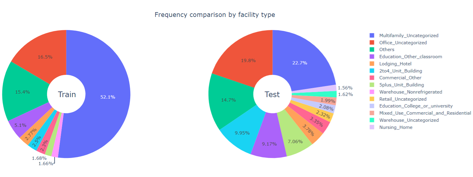
Observations
- In the training data, more than \(52\%\)
of the buildings are
Multifamily_Uncategorizedand at a distant second, \(16.5\%\) of the buildings areOffice_Uncategorized - In the test data, the distribution is more evenly spread out with
Multifamily_UncategorizedandOffice_Uncategorizedrespectively taking up \(22.7\%\) and \(19.8\%\) of the observations
Multivariate Analysis
First, we explore relationships among the predictor variables. In the univariate analysis, we had compared the frequency of observations by state and building class separately. Now we check the same comparison jointly. In particular, we examine it by state for each building class.
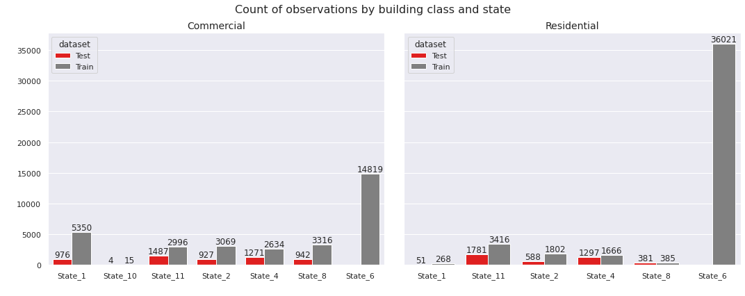
Observations
- The data from
State_10only contains commercial buildings
The univariate analysis showed that Multifamily_Uncategorized and Office_Uncategorized make up majority of the buildings in both the training data and the test data.
Clearly, Multifamily_Uncategorized buildings are mostly residential whereas the Office_Uncategorized buildings are mostly commercial. So we examine the facility types separately for residential and commercial buildings.
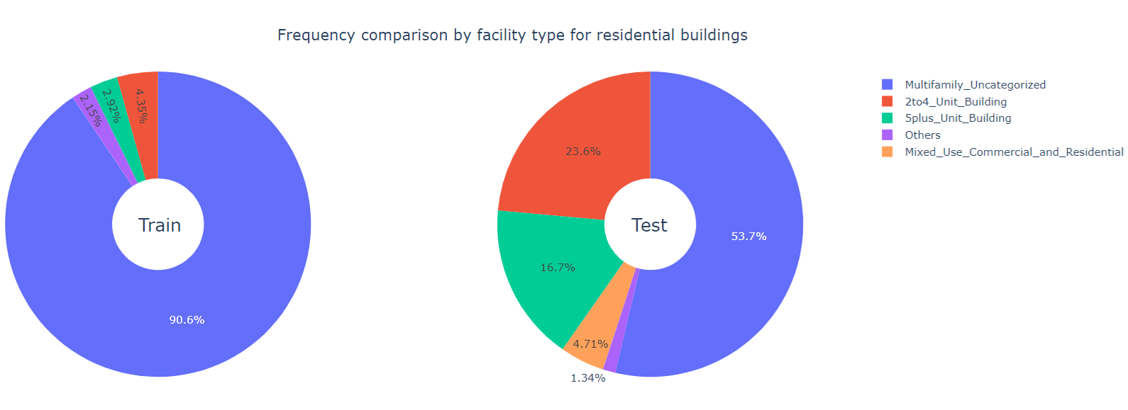
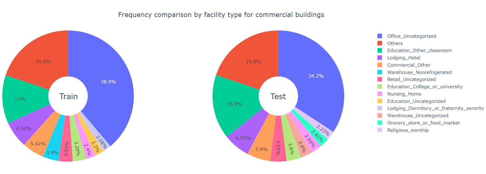
We observe that majority of the residual buildings fall into the Multifamily_Uncategorized facility type, while most of the commercial buildings has the Office_Uncategorized facility type.
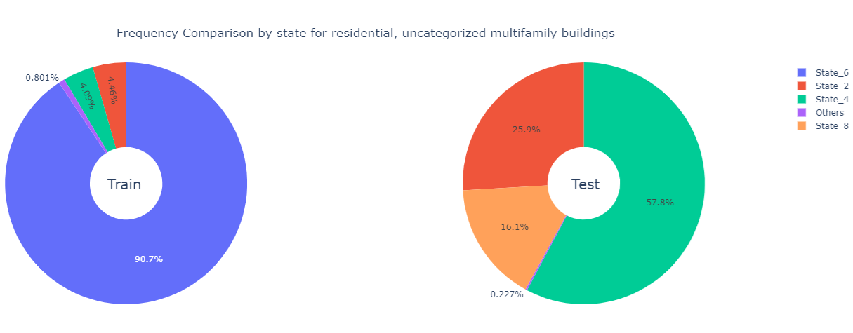
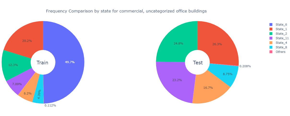
We focus on these two categories with the specific building class type that they dominate and perform a state-level frequency comparison.
Observations
- Over \(90\%\)
of the residential buildings in the training data are
Multifamily_Uncategorized - Over \(90\%\)
of the residential, uncategorized multifamily buildings in the
training datacome fromState_6 - Over \(50\%\)
of the residential buildings in the test data are
Multifamily_Uncategorized - Over \(50\%\)
of the residential, uncategorized multifamily buildings in the test data come from
State_4 - Over one-third of the commercial buildings in both the training set and the test data are
Office_Uncategorized - Almost half of the commercial, uncategorized office buildings in the training data come from
State_6
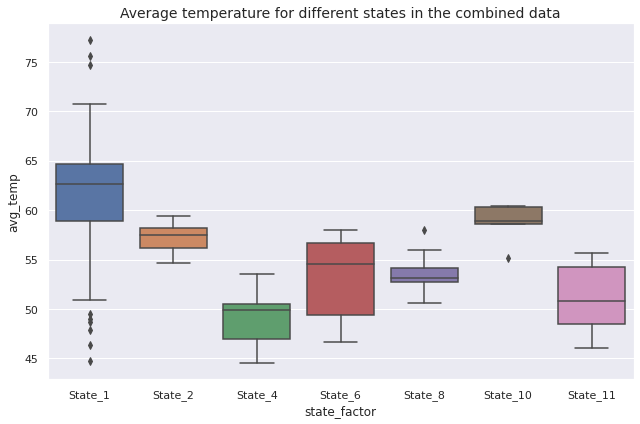
Next, we compare the distributions of average temperature for different states in the combined data through boxplots.
Observations
State_1has the highest average temperature andState_4has the lowest average temperatureState_6,State_11,State_1andState_4have greater dispersion thanState_2,State_8andState_10
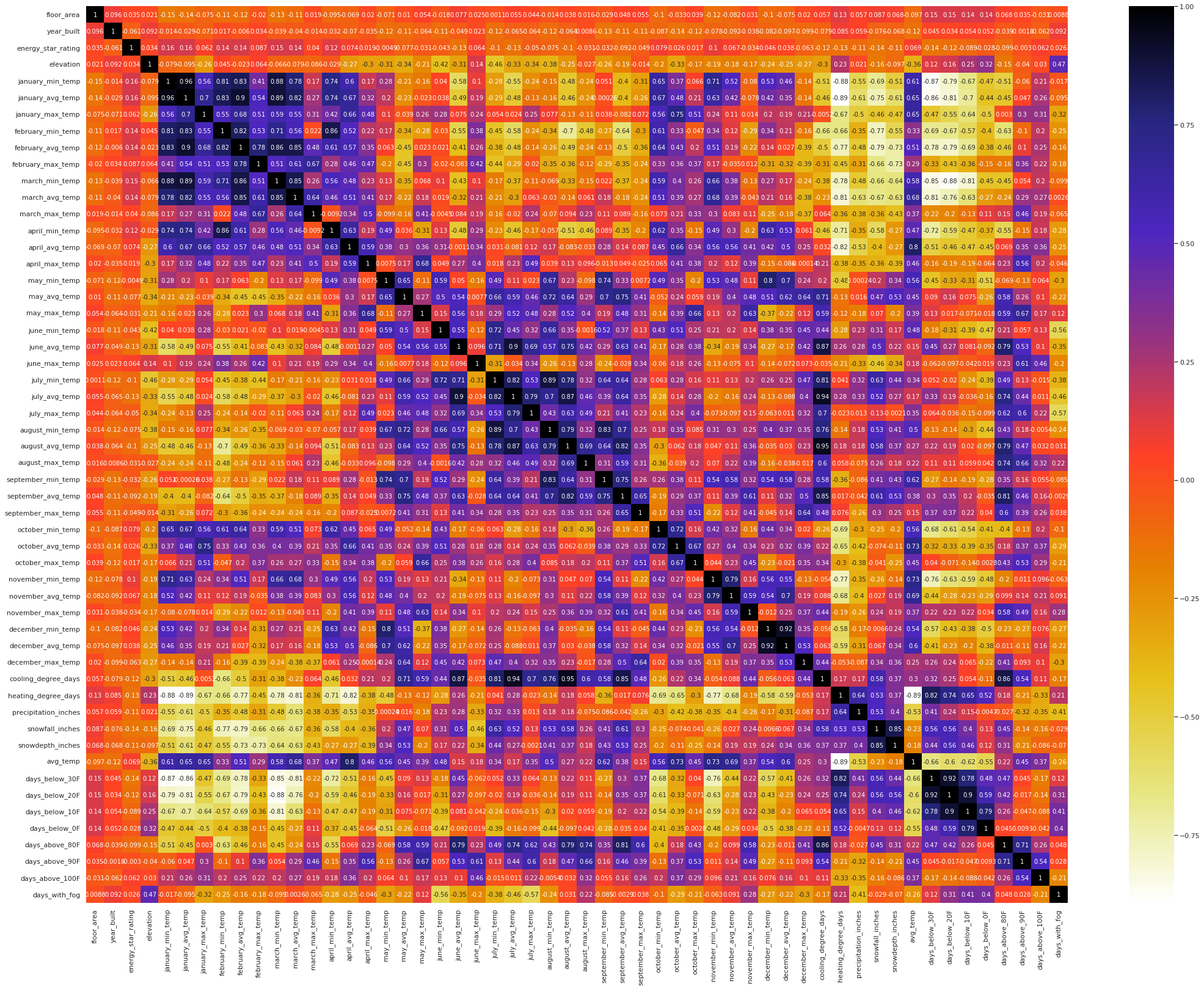
Now we examine the correlation structure among numerical features through a correlation heatmap.
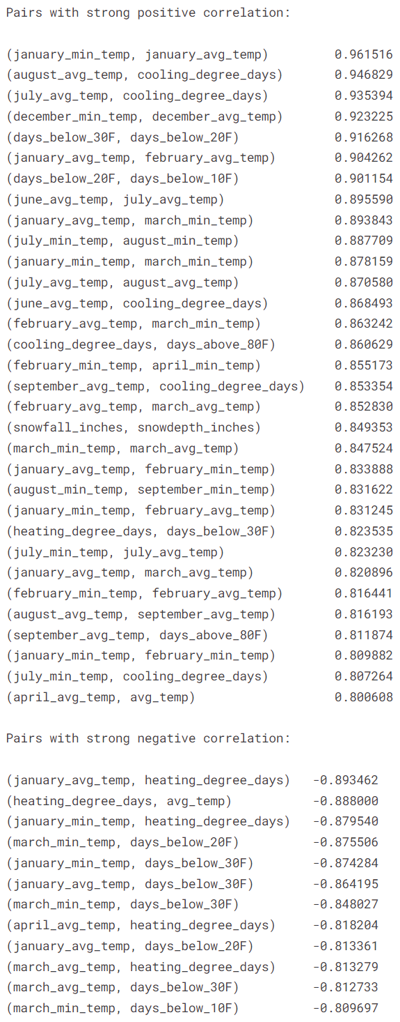
Next, we produce a list of pairs of features with correlation coefficient higher than \(0.8\) or lower than \(-0.8\).
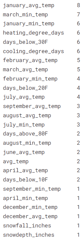
We detect the variables that appear the most in this list of pairs of features with strong correlation.
Observations
- The heatmap suggests strong level of multicollinearity among the numerical features
- There are \(32\) pairs of feature with correlation coefficient over \(0.8\) and \(12\) pairs of feature with correlation coefficient below \(-0.8\)
- There are \(7\) pairs of features with correlation coefficient over \(0.9\)
- The features
january_avg_temp,march_min_temp,january_min_temp,heating_degree_days,days_below_30Fandcooling_degree_daysare involved in more than \(5\) pairs of features with absolute value of correlation coefficient over \(0.8\)
Next, we investigate the relationships of the target variable with the predictor variables. For categorical variables like year_factor, state_factor, and building_class, we present histograms of the target variable site_eui for each categories.

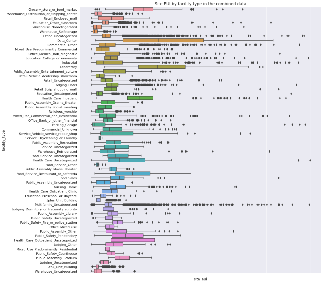
Next, we compare the overall distributions of site_eui for different facility type in the combined data through horizontal boxplots.
Observations
site_euiforGrocery_store_or_food_market,Data_Center,Laboratory,Health_Care_Inpatient,Health_Care_Uncategorized,Health_Care_Outpatient_Uncategorized,Food_Service_Restaurant_or_cafeteria,Public_Safety_Penitentiaryare relatively larger than the rest of the facility typessite_euiforData_Center,Laboratory,Service_Vehicle_service_repair_shop,Health_Care_Uncategorized,Health_Care_Outpatient_Uncategorized,Food_Service_Restaurant_or_cafeteriahave more dispersion than other facility types
Next, we observe the overall relationship of the target variable with the numerical features through scatterplots.

Observations
- Majority of the data points correspond to the lower values of
floor_areas,elevation,cooling_degree_days,snowfall_inches,snowdepth_inches,days_above_90F - Majority of the data points correspond to the higher values of
year_built - The weather related numerical columns do not appear to have any strong relationship with
site_eui
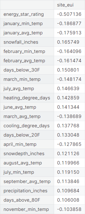
We summarize the linear relationship between the target variable and the numerical features through corresponding correlation coefficient.
Observations
- The target variable
site_euihas moderately strong negative correlation withenergy_star_rating - It has weak positive correlation with
snowfall_inches,days_below_30F,july_avg_temp,heating_degree_days,june_avg_temp,cooling_degree_days,days_below_20F,snowdepth_inches,august_avg_temp,july_min_temp,september_avg_temp,precipitation_inches,days_above_80F - It has weak negative correlation with
january_min_temp,january_avg_temp,february_min_temp,february_avg_temp,march_min_temp,march_avg_temp,april_min_temp,november_min_temp - It does not show any significant linear relationship with
days_below_10F,february_max_temp,april_avg_temp,october_min_temp,september_max_temp,july_max_temp,august_min_temp,may_avg_temp,january_max_temp,floor_area,december_max_temp,avg_temp,december_min_temp,november_avg_temp,days_below_0F,may_max_temp,days_with_fog,june_min_temp,december_avg_temp,september_min_temp,june_max_temp,october_max_temp,elevation,august_max_temp,march_max_temp,november_max_tempandoctober_avg_temp
○ Data Preprocessing
Missing Data Imputation
In basic data exploration, we have seen that:
- The training data contains more than \(50\%\)
missing values for the features
days_with_fog,direction_peak_wind_speed,direction_max_wind_speedandmax_wind_speed - The test data contains more than \(88\%\) missing values for the same features
Hence we drop these features.
- The feature
energy_star_ratinghas \(35.25\%\) missing values in the training data and \(23.22\%\) missing values in the test data - The feature
year_builthas \(2.42\%\) missing values in the training data and \(0.94\%\) missing values in the test data
We impute the missing values not only for year_built, which has a minimal amount of missing values, but also for energy_star_rating, considering the fact that it has the highest correlation (in absolute value) with the target variable.
In the training set:
energy_star_ratingis missing for \(26709\) observationsyear_builtis missing for \(1837\) observations- Exactly one between these two features is missing for \(26078\) observations
- Both features are missing for \(1234\) observations
- In total, \(27312\) observations contain missing data
In the test set:
energy_star_ratingis missing for \(2254\) observationsyear_builtis missing for \(92\) observations- Exactly one between these two features is missing for \(2262\) observations
- Both features are missing for \(42\) observations
- In total, \(2304\) observations contain missing data
Both energy_star_rating and year_built are numerical features. We opt for median imputation to negate the effect of possible outliers. First, we implement the imputation on the training set. Then, we impute the missing values of energy_star_rating and year_built in the test data by the medians of the respective features in the training data (not the test data), following the suggestion of Aurélien Géron in his book Hands-On Machine Learning with Scikit-Learn and TensorFlow (page \(60\),
chapter \(2\)):
… you should compute the median value on the training set, and use it to fill the missing values in the training set, but also don’t forget to save the median value that you have computed. You will need it later to replace missing values in the test set when you want to evaluate your system, and also once the system goes live to replace missing values in new data.
Categorical Data Encoding
We employ target encoder to numerically encode the categorical features state_factor, building_class and facility_type. In the present situation, the target variable (site_eui) is a continuous variable. According to this documentation on target encoder:
For the case of continuous target: features are replaced with a blend of the expected value of the target given particular categorical value and the expected value of the target over all the training data.
First, we encode the categorical columns in the training data. The following code snippet encodes a single column col of a training set df_train with target variable target into the column col_encoded.
encoder = TargetEncoder()
df_train[col_encoded] = encoder.fit_transform(df_train[col], df_train[target])
The mapping of the original values and the corresponding encoded values for each categorical feature in the training data are recorded in form of dictionaries. Implementation for a single column:
col_enc_dict = {}
for i in range(len(df_train[col].unique())):
    col_enc_dict[df_train[col].unique().tolist()[i]] = df_train[col_encoded].unique().tolist()[i]
We encode the categorical columns in the test data, using dictionaries containing the exact encoding scheme (the map connecting original values and encoded values) of the same columns in the training data.
df_test[col_encoded] = df_test[col].map(col_enc_dict)
Subsequently, we drop the original categorical columns from the training set and the test set.
○ Feature Engineering
- Extraction of new features
- Exploratory data analysis of the new features
- Transformation
- Binarization
Extraction of new features
We compress the monthly weather statistics into seasonal weather statistics. This reduces the number of features greatly without losing significant information. First, we separate out the columns corresponding to monthly temperature statistics into four lists corresponding to four seasons.
temp_all = [col for col in data_train.columns if "temp" in col]
temp_winter = [col for col in temp_all if ('january' in col or 'february' in col or 'december' in col)]
temp_spring = [col for col in temp_all if ('march' in col or 'april' in col or 'may' in col)]
temp_summer = [col for col in temp_all if ('june' in col or 'july' in col or 'august' in col)]
temp_autumn = [col for col in temp_all if ('september' in col or 'october' in col or 'november' in col)]
Next, we extract the seasonal temperature statistics out of the monthly temperature statistics from the training DataFrame data_train. Also, we convert cooling_degree_days and heating_degree_days from yearly scale to monthly scale.
data_train['min_temp_winter'] = data_train[temp_winter].min(axis = 1)
data_train['max_temp_winter'] = data_train[temp_winter].max(axis = 1)
data_train['avg_temp_winter'] = data_train[temp_winter].mean(axis = 1)
data_train['std_temp_winter'] = data_train[temp_winter].std(axis = 1)
data_train['skew_temp_winter'] = data_train[temp_winter].skew(axis = 1)

(similarly for temp_spring, temp_summer, and temp_autumn)

data_train['cooling_degree_days_per_month'] = data_train['cooling_degree_days'] / 12
data_train['heating_degree_days_per_month'] = data_train['heating_degree_days'] / 12
We repeat the same feature extraction procedure for the test data. In total, we have generated \(22\) new features from the pool of \(39\) original weather related features. Finally, we drop the old weather related features from the training set and the test set.
Exploratory data analysis of the new features
Understanding the new features
We convert the month-based temperature related features to season-based features by partitioning the full year into four seasons: winter (December, January, February), spring (March, April, May), summer (June, July, August) and spring (September, October, November).
- min_temp_winter: minimum temperature in winter (in Fahrenheit) at the location of the building
- max_temp_winter: maximum temperature in winter (in Fahrenheit) at the location of the building
- avg_temp_winter: average temperature in winter (in Fahrenheit) at the location of the building
- std_temp_winter: standard deviation of temperature in winter (in Fahrenheit) at the location of the building
- skew_temp_winter: skewness of temperature in winter (in Fahrenheit) at the location of the building
(Similarly for spring, summer and autumn)
- cooling_degree_days_per_month: average number of degrees where the daily average temperature exceeds \(65\) degrees Fahrenheit in a month
- heating_degree_days_per_month: average number of degrees where the daily average temperature falls under \(65\) degrees Fahrenheit in a month
We list the extracted features along with their corresponding datatype.
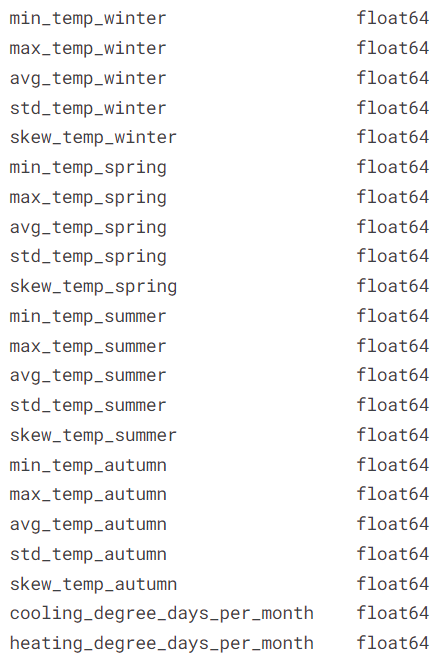
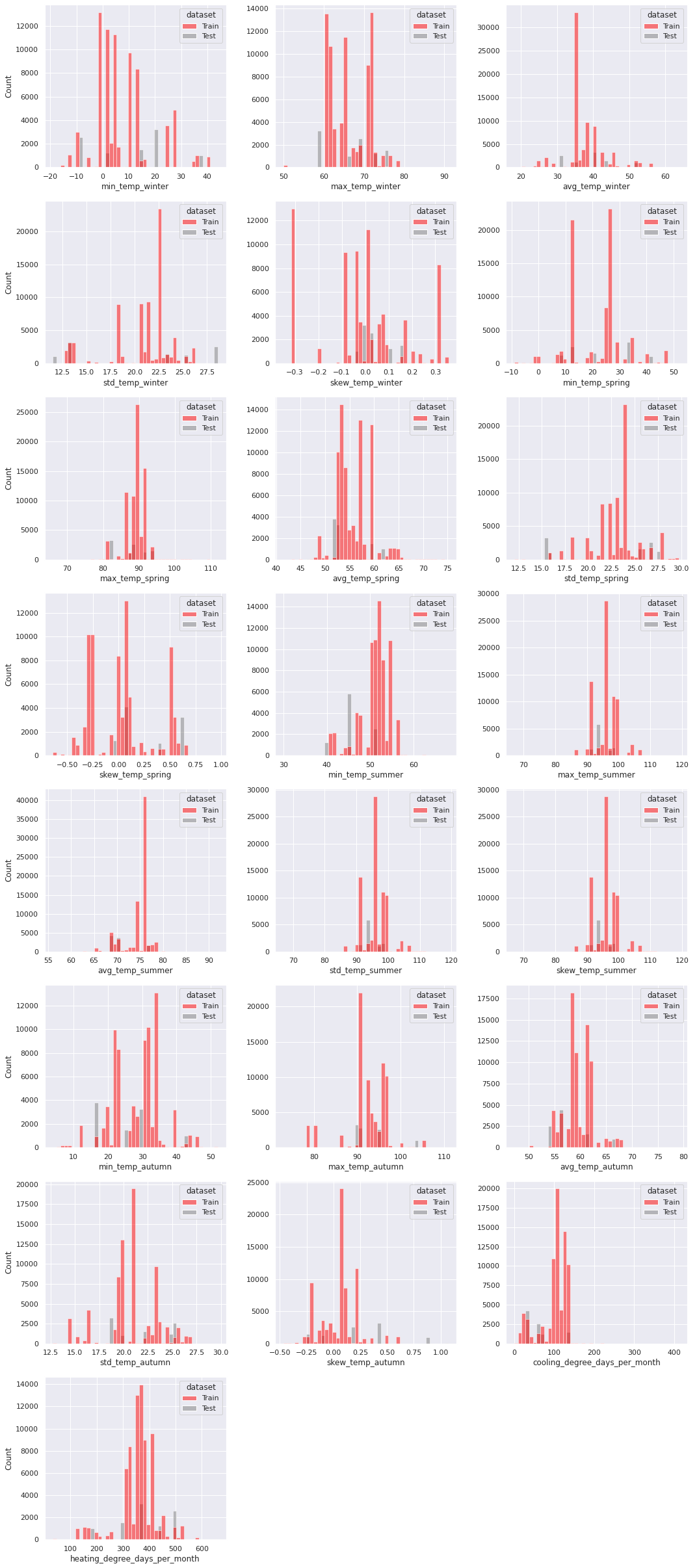
We present the distribution of the new features through histograms.
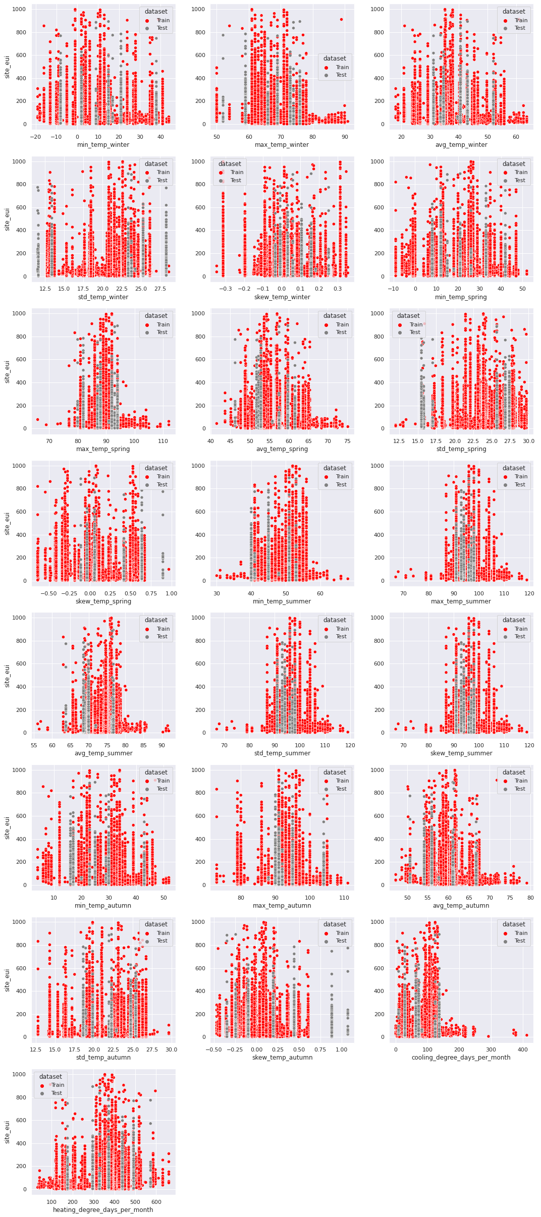
Next, we check the relationship of Site EUI with the new features through scatterplots.
Transformation
We apply location change \(x \mapsto x - min(x) + 1\)
on the features floor_area and elevation to make their range start from \(1\).
The relocated variables fall inside the range \([1, \infty)\).
Implementation on a single column col of a training set df_train and a test set df_test:
min_ = df_train[col].min()
df_train[col] = df_train[col].apply(lambda x: x - min_ + 1)
df_test[col] = df_test[col].apply(lambda x: x - min_ + 1)
Now, we apply the log transformation \(y \mapsto \log{y}\). Implementation on a single column:
df_train[col] = df_train[col].apply(np.log)
df_test[col] = df_test[col].apply(np.log)
The relocation preceding the log transformation ensures that there are no negative values to be fed to the \(\log\) function. The addition of \(1\) ensures that there are no values very close to \(0\), which the log transformation maps to extreme negative values.
Note that we use the same \(\min(x)\) from the training data in the test data, to keep the transformation same for the two datasets.
Binarization
The univariate analysis showed that the features days_above_100F and days_above_110F are \(0\)
for most observations in both the training data and the test data. So we binarize the two features, keeping the zero values as \(0\)
and mapping the non-zero values to \(1\).
Implementation on a single column col of a training set df_train and a test set df_test:
df_train[col] = np.where(df_train[col] == 0, 0, 1)
df_test[col] = np.where(df_test[col] == 0, 0, 1)
○ Baseline Modeling
In this section, we use three algorithms, namely random forest, XGBoost, and CatBoost to the problem at hand and compare their baseline performances.
We begin by typecasting the numerical features to float64. Then, we split the predictor variables and the target variable out of the datasets. Also, we drop the column building_id from both the training set and the test set as it does not contribute to the prediction of the target variable.
Random Forest
rf = RandomForestRegressor(random_state = 0)
The baseline performance of Random Forest algorithm is summarized below.

XGBoost
xgb = XGBRegressor(random_state = 0)
The baseline performance of XGBoost algorithm is summarized below.

CatBoost
catb = CatBoostRegressor(
    iterations = 1000,
    learning_rate = 0.02,
    depth = 12,
    eval_metric = 'RMSE',
    random_state = 0,
    bagging_temperature = 0.2,
    od_type = 'Iter',
    metric_period = 100,
    od_wait = 100
)
The baseline performance of CatBoost algorithm is summarized below.

Model Comparison
We compare the models based on cross-validation scores through categorical plots.

Observation: Based on all three evaluation metrics, the cross-validation scores suggest that the random forest regressor is working the best, followed by the XGBoost regressor, and then the CatBoost regressor.
○ Hyperparameter Tuning
Hyperparameters and Optuna
We apply hyperparameter tuning on the random forest algorithm, which is performing best among the three baseline candidates. For this purpose, we use the Optuna framework.
In particular, we optimize the following hyperparameters:
n_estimators(integer): The number of trees in the forestmax_depth(integer): The maximum depth of the treemin_samples_split(integer): The minimum number of samples required to split an internal nodemax_features(float): The proportion of features to consider when looking for the best split
Objective Function
We define the objective function.
def objective_rf(trial, data = X_train, target = y_train):
    param = {
        "n_estimators": trial.suggest_int("n_estimators", 100, 500),
        "max_depth": trial.suggest_int("max_depth", 5, 20),
        "min_samples_split": trial.suggest_int("min_samples_split", 2, 10),
        "max_features": trial.suggest_float("max_features", 0.01, 0.95)
    }
    model = RandomForestRegressor(**param)
    kfolds = KFold(n_splits = 6, shuffle = True)
    scores = cross_val_score(model, data, target, cv = kfolds, scoring = "neg_root_mean_squared_error")
    return -scores.mean()
Tuning Function
We build the tuning function.
def tuner(objective, n = 10, direction = 'minimize'):
    sampler = optuna.samplers.TPESampler(seed = 0)
    study = optuna.create_study(direction = direction, sampler = sampler)
    study.optimize(objective, n_trials = n)
    display(optuna.visualization.plot_optimization_history(study))
    best_params = study.best_params
    best_score = study.best_value

    print(f"Best RMSE score: {best_score}")
    print(f"Optimized parameters: {best_params}\n")
    print("-------- Tuning complete --------")

    return best_params, best_score
Tuner Search and Model Fitting
We tune the parameters using the tuner function.
rf_param, rf_score = tuner(objective_rf, n = 10, direction = 'minimize')
The cross-validation RMSE scores for each trial of the tuning process are plotted to visualize the optimization history.
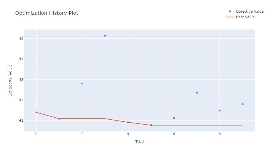
Best RMSE score: \(40.76934266775879\)
Optimized hyperparameters:
n_estimators: \(492\)max_depth: \(17\)min_samples_split: \(6\)max_features: \(0.7436974257092681\)
We fit the tuned model on the entire training set.
○ Prediction and Evaluation
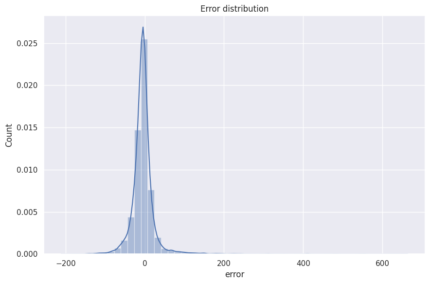
We use the fitted model to predict on the test set and visualize the error distribution.
The performance of the Random Forest algorithm with optimized hyperparameters is summarized below.

○ Acknowledgements
- Hands-On Machine Learning with Scikit-Learn and TensorFlow by Aurélien Géron
- WiDS Datathon 2022 Dataset
○ References
- Annotation
- Box plot
- CatBoost
- Categorical data encoding
- Coefficient of determination
- Continuous variable
- Correlation
- Cross-validation
- Data preprocessing
- Data transformation
- Energy usage intensity
- Exploratory data analysis
- Feature engineering
- Heat map
- Histogram
- Hyperparameter optimization
- Imputation
- Logarithm
- Mean absolute error
- Missing data
- Multicollinearity
- Optuna
- Random forest
- Relational plot
- Root mean square deviation
- Scatter plot
- Target encoder
- Test set
- Training set
- XGBoost