Road Traffic Accidents Severity Classification
The severity of road traffic accidents can be influenced by several factors, including the various attributes of the vehicles involved, the drivers, the casualties, and the surrounding conditions. The objective of the project is to build a prediction model to classify the severity of road traffic accidents into a hierarchy consisting of three categories, namely slight injury, serious injury, and fatal injury, based on the information on the pertinent attributes.
○ Contents
- Overview
- Introduction
- Exploratory Data Analysis
- Data Preprocessing
- Baseline Models
- Hyperparameter Tuning
- Prediction and Evaluation
- Acknowledgements
- References
○ Overview
- The severity of road traffic accidents may depend on several factors, including the attributes of the involved vehicles, drivers, casualties, and surrounding conditions.
- In this project, we aim to predict the severity of an accident in terms of a given hierarchy (slight, serious, and fatal), with the help of information on the relevant attributes.
- A detailed exploratory data analysis on the dataset is carried out.
- The observations obtained from EDA are used in the data preprocessing stages.
- We employ decision tree, random forest, XGBoost, and ExtraTrees classifiers to predict the severity of an accident as slight, serious, or fatal.
- We apply hyperparameter tuning to the XGBoost classifier, which appears to perform best among the baseline candidates. We also tune the ExtraTrees classifier and the random forest classifier, as their performance is very close to that of the XGBoost classifier.
- The final model obtains a weighted \(F_1\)-score of \(0.795060\) on the test set.
○ Introduction
Data
The dataset used in the project has been prepared from manual records of road traffic accidents in the years \(2017-2020\) , collected from Addis Ababa sub city police departments. Sensitive information have been excluded during the data encoding process. The final dataset has information on \(12316\) accidents, each with \(32\) attributes.
Project Objective
The aim of the project is to build prediction models, based on these factors, to classify the severity of accidents into three categories:
- Slight injury
- Serious injury
- Fatal injury
Thus, it is a multiclass classification problem.
Evaluation Metric
Precision and recall are universally accepted metrics to capture the performance of a model, when restricted respectively to the predicted positive class and the actual positive class. Let us denote
- TP: Number of true positives
- TN: Number of true negatives
- FP: Number of false positives
- FN: Number of false negatives
In terms of these quantities, Precision and Recall are defined as
The \(F_1\)-score provides a balanced measuring stick by considering the harmonic mean of the above two metrics.
For its equal emphasis on both precision and recall, \(F_1\)-score is one of the most suitable metrics for evaluating the models in this project.
In the dataset, we have a target variable (Accident_severity) that takes three possible values, essentially partitioning the dataset into three target classes. This can be converted to a binary partition by considering one class as the positive class and the rest two combined as the negative class. Now this positive-negative partition can be done from the perspective of each target class, producing three \(F_1\)-scores.
We take the weighted \(F_1\)-score
, which is the average of these three scores weighted by the number of true instances for each class, as an evaluation metric to assess the models.
○ Exploratory Data Analysis
Summary of the Data
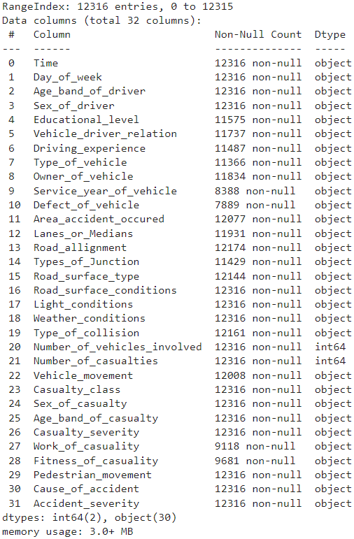
Data Synopsis
- Number of observations: \(12316\)
- Number of columns: \(32\)
- Memory Usage: \(3.0+\) MB
- Number of integer columns: \(2\)
- Number of object columns: \(30\)
- Number of columns with missing values: \(16\)
- Columns with missing values:
Educational_level,Vehicle_driver_relation,Driving_experience,Type_of_vehicle,Owner_of_vehicle,Service_year_of_vehicle,Defect_of_vehicle,Area_accident_occured,Lanes_or_Medians,Road_allignment,Types_of_Junction,Road_surface_type,Type_of_collision,Vehicle_movement,Work_of_casuality,Fitness_of_casuality
The Target Variable
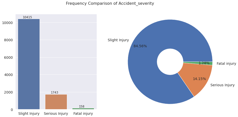
The charts show that the data is imbalanced with respect to the target variable Accident_severity. Note that the percentage values in the pie chart is rounded off to two decimal places and hence may not add up to exactly \(100\%\)
. The class of accidents with slight injury is the majority class with \(84.56\%\)
of the instances falling in that category. The class of accidents with serious injury comes next with a proportion of \(14.15\%\)
. The class of accidents with fatal injury contributes only \(1.28\%\)
of the entirety of the dataset. Next we explore various feature variables in the dataset with a particular goal of identifying how the target variable behaves in relation to variation in these features.
Time
To examine the distribution of time, we convert the feature from \(hh:mm:ss\) format to seconds with the mapping
def convert_to_seconds(x):
    hh = int(x.split(':')[0])
    mm = int(x.split(':')[1])
    ss = int(x.split(':')[2])
    time_in_ss = (hh * 60 * 60) + (mm * 60) + ss
    return time_in_ss
Under this mapping, the range of time is \(0\) to \(86400\) . We show the conversion for five specific, equispaced time points (the first and last of which are \(24\) hours apart, but coincides in the cyclic scale).
- \(00:00:00 \to 0\) (\(12\) a.m.)
- \(06:00:00 \to 21600\) (\(6\) a.m.)
- \(12:00:00 \to 43200\) (\(12\) p.m.)
- \(18:00:00 \to 64800\) (\(6\) p.m.)
- \(24:00:00 \to 86400\) (next day \(12\) a.m.)
In the histograms, each bin denotes one-hour time interval, starting from \(12\) a.m. We convert the time labels back to the usual notation with a.m. and p.m. for better understanding of the distribution.
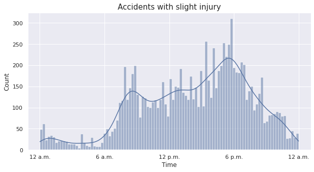
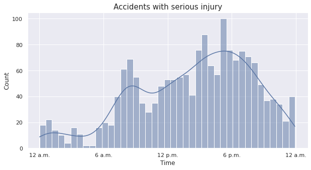
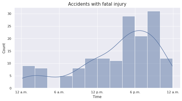
The distribution reflects the intuition that there are more traffic accidents in the day time than at night. In particular, for accidents with slight or serious injuries, the distribution appears to have a bimodal structure with a distinct local mode apart from the global mode. It rises sharply from \(5\) a.m. - \(6\) a.m. until it reaches the local peak at \(8\) a.m. - \(9\) a.m. After troughing slightly, it gradually rises to the global modal class \(5\) p.m. - \(6\) p.m. Then it falls sharply before stabilizing around \(12\) a.m. - \(1\) a.m. and stays low until \(5\) a.m. - \(6\) a.m. For accidents with fatal injuries, however, the distribution appears to be slightly different from the former two cases, with a global peak in \(8\) p.m. - \(10\) p.m. and a separate local peak in \(4\) p.m. - \(6\) p.m.
Other Features
We present categorical plots to compare frequency distributions of other features across target classes in this notebook. Example:
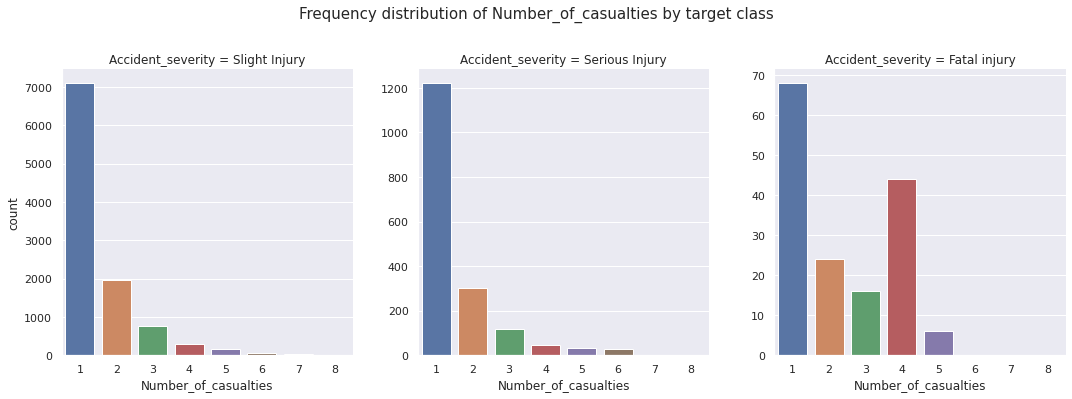
We denote:
- target class 1: class of accidents with slight injury
- target class 2: class of accidents with serious injury
- target class 3: class of accidents with fatal injury
Then we observe:
-
Features that have more or less similar distribution for all target classes:
Sex_of_driver,Educational_level,Vehicle_driver_relation,Owner_of_vehicle,Defect_of_vehicle,Road_surface_type,Road_surface_conditions,Light_conditions,Weather_conditions,Vehicle_movement,Sex_of_casualty,Casualty_severity,Fitness_of_casuality,Pedestrian_movement -
Features that have more or less similar distribution for target class 1 and target class 2, but have a different distribution for target class 3:
Day_of_week,Driving_experience,Service_year_of_vehicle,Area_accident_occured,Lanes_or_Medians,Road_allignment,Types_of_Junction,Type_of_collision,Number_of_casualties,Casualty_class,Age_band_of_casualty,Work_of_casuality,Cause_of_accident -
Features that have more or less similar distribution for target class 2 and target class 3, but have a different distribution for target class 1:
Number_of_vehicles_involved -
Features that have different distributions for all target class:
Age_band_of_driver,Type_of_vehicle
○ Data Preprocessing
- Outlier Detection
- Combining Similar Values
- Missing Data Imputation
- Categorical Data Encoding
- Predictor-Target Split
- Train-Validation-Test Split
- Feature Scaling
- Resampling
- Feature Selection
Outlier Detection
There are three numerical variables in the dataset.
Timeis a bounded variable. After the convertion, it is strictly bounded between \(0\) and \(86400\) . It has a minimum value of 60 and a maximum of \(86340\) . Since we know that the traffic are active round the clock (even with the obvious bias to day-time), we discard the possibility of outliers here.Number_of_vehicles_involvedis a count data, taking positive integer values (as there can be no traffic accident without vehicles).Number_of_casualtiesis again a count data, taking positive integer values.
We present the respective boxplots to check for outliers.
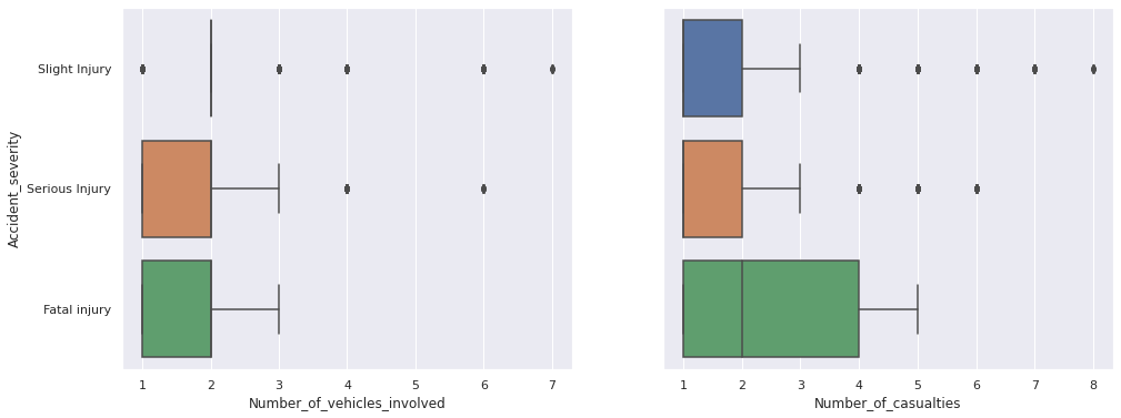
Despite the appearances of the apparent outliers, we refrain from deleting or modifying them as it is evident from the range of the variables that these are most likely to be genuine values, containing relevant information about the corresponding variables.
Combining Similar Values
We combine certain similar categories that appear in the dataset. For instance, 5 and Under 18 are two categories of the feature Age_band_of_casualty. These two categories can be combined for all practical purposes, as one is a subset of the other.
def combine_similar(data):
    data_out = data.copy(deep = True)
    data_out = data_out.replace('Unknown', 'unknown')
    data_out = data_out.replace('Other', 'other')
    data_out = data_out.replace('Unknown or other', 'other')
    data_out = data_out.replace('Darkness - lights unlit', 'Darkness - no lighting')
    data_out['Age_band_of_casualty'] = data_out['Age_band_of_casualty'].replace('5', 'Under 18')
    return data_out
Missing Data Imputation
Columns with missing values (sorted by count):
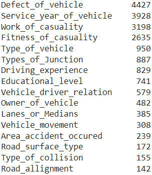
\(16\) columns (out of \(32\) ) contain missing values. All features with missing values are categorical in nature.
Proportional imputation: With the goal of keeping the feature distributions same before and after imputation, we impute the missing values in a column in such a way so that the proportions of the existing unique values in the column remain roughly same as those were prior to the imputation.
def prop_imputer(data):
    data_prop = data.copy(deep = True)
    missing_cols = data_prop.isna().sum()[data_prop.isna().sum() != 0].index.tolist()
    for col in missing_cols:
        values_col = data_prop[col].value_counts(normalize = True).index.tolist()
        probabilities_col = data_prop[col].value_counts(normalize = True).values.tolist()
        data_prop[col] = data_prop[col].fillna(pd.Series(np.random.choice(values_col, p = probabilities_col, size = len(data))))
    return data_prop
Examples of frequency distributions of features before and after implementing proportional imputation:
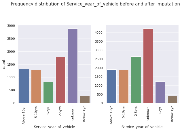
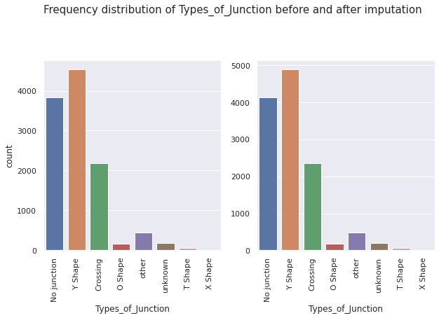
As expected, we observe that while the frequencies change, the overall distributions of the features remain the same before and after applying proportional imputation.
Categorical Data Encoding
After convertion of time from \(hh:mm:ss\) to seconds format, the dataset contains
- \(3\) integer variables
- \(29\) categorical variables
Categorical variables can be ordinal (ordered, e.g. very bad, bad, good, very good) or nominal (unordered, e.g. red, blue, yellow, green). We observe that in the dataset, the following categorical variables are ordinal.
Age_band_of_driverEducational_levelDriving_experienceService_year_of_vehicleLight_conditionsAge_band_of_casualtyCasualty_severityAccident_severity
The rest of the categorical variables are nominal. An appropriate encoding scheme is given as follows:
- Ordinal features \(\to\) Manual encoding or Label encoding
- Nominal features \(\to\) One-hot encoding
However, the dataset contains a lot of nominal features. As a result one-hot encoding produces too many columns, which eventually leads to curse of dimensionality and loss of relevant information at the feature selection stage. For this reason, we resort to the following scheme:
- Ordinal features \(\to\) Manual encoding
- Nominal features \(\to\) Label encoding
The manual encoding of ordinal features involves mapping the categories to integers while maintaining the order. For instance, the categories of the feature Light_conditions are mapped in the following way.
Darkness - no lighting\(\to 1\)Darkness - lights lit\(\to 2\)Daylight\(\to 3\)
The notebook contains the code for implementing manual encoding to several ordinal features simultaneously. This is done in three steps:
- Creating dictionary of mapping for each ordinal variable
- Creating a dictionary with keys as variable names and values as the corresponding dictionary of mapping created in step 1
- Defining a function for implementing manual encoding using the dictionary of all mappings created in step 2
The function to implement label encoding to selected columns of an input DataFrame is given as follows.
def label_encoder(data, cols):
    data_le = data.copy(deep = True)
    le = LabelEncoder()
    for col in cols:
        data_le[col] = le.fit_transform(data_le[col])
    return data_le
The encoding scheme is implemented on the features, leaving the target variable as it is for the time being. The features data is now completely in numerical format, allowing us to examine the correlation structure of the features through a heatmap. While the color-coding gives a rough idea, one may have to open the image in a new tab and zoom to check the numerical values.
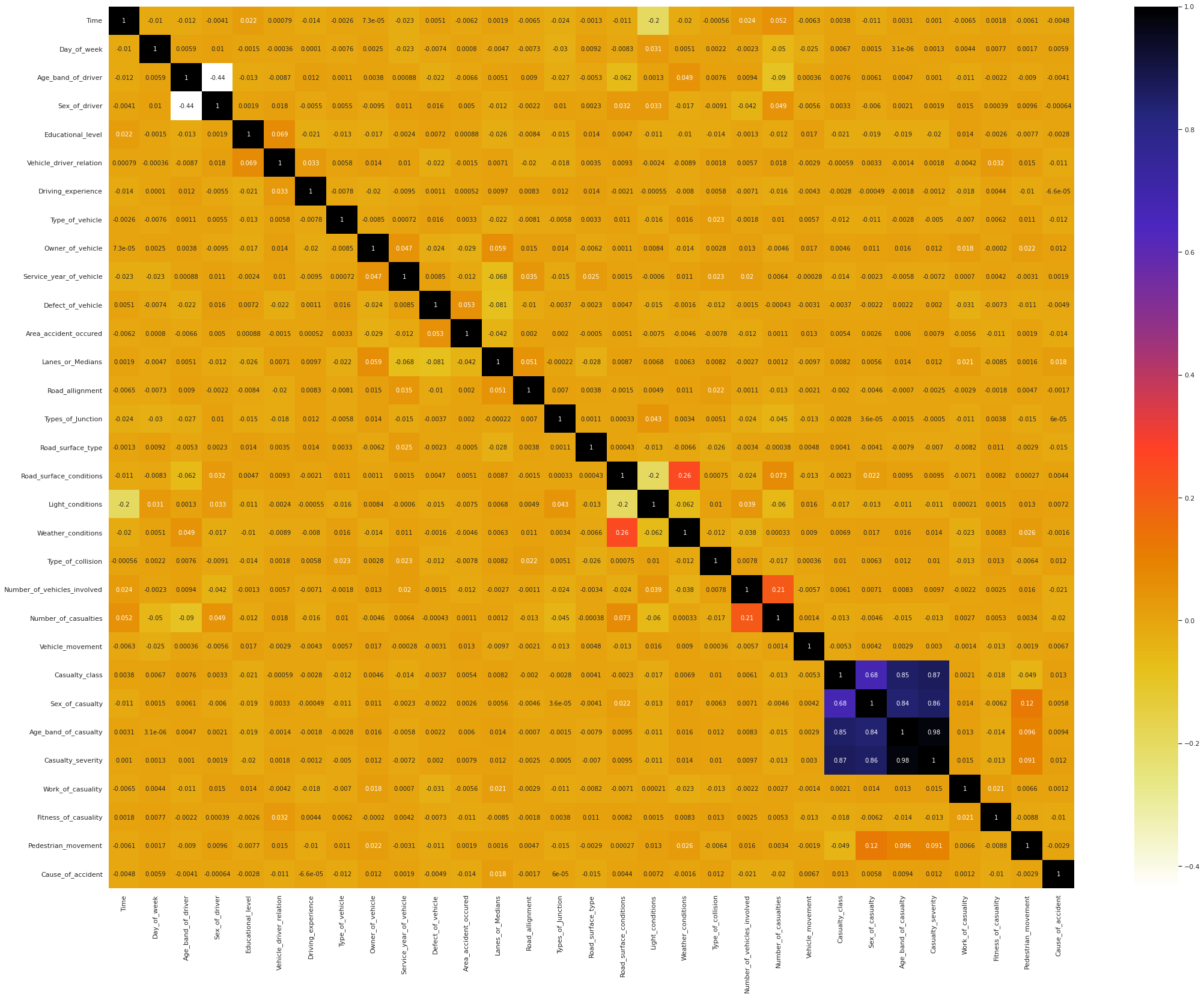
We observe that the features Casualty_class, Sex_of_casualty, Age_band_of_casualty, and Casualty_severity are highly correlated. We keep Age_band_of_casualty and drop the other three features.
Predictor-Target Split
At this stage, we split the target variable from the independent variables using the following function.
def predictor_target_split(data, target):
    X = data.drop(target, axis = 1)
    y = data[target]
    return X, y
Train-Validation-Test Split
Then we split the dataset into a training set, a validation set, and a test set in \(80:10:10\) ratio using the train_test_split function.
X_train, X_test, y_train, y_test = train_test_split(X, y, stratify = y, test_size = 0.2, shuffle = True, random_state = 0)
X_valid, X_test, y_valid, y_test = train_test_split(X_test, y_test, stratify = y_test, test_size = 0.5, shuffle = True, random_state = 0)
Feature Scaling
The converted Time takes huge values and is likely to distort the training procedure. We consider a modified version of the min-max normalization. The original transformation is given as:
We modify the transformation a bit to incorporate a scaling factor \(c\)
, so that the rescaled Time variable has the range \([0, c]\)
, whenever its maximum value exceeds \(c\)
.
The next function implements this idea with slight modifications. Due to the well-defined bounds of the time variable, we replace \(\min{\left(x\right)}\) and \(\max{\left(x\right)}\) respectively by \(0\) and \(24 \times 60 \times 60\).
def normalize_time(data, c = 1):
    data_normalized = data.copy(deep = True)
    if 'Time' in data_normalized.columns:
        if data_normalized['Time'].max() > c:
            data_normalized['Time'] = c * data_normalized['Time'] / (24*60*60)
    return data_normalized
We normalize the Time variable with the scaling factor \(c\)
set at \(10\),
i.e. the time (in seconds) is normalized to the scale of \(0-10\),
keeping the values to a similar scale as of the other variables.
Resampling
The next function implements the synthetic minority over-sampling technique (SMOTE) to balance out the training set with respect to the target variable.
def smote(X_train, y_train):
    smote = SMOTE()
    X_train_smote, y_train_smote = smote.fit_resample(X_train, y_train)
    return X_train_smote, y_train_smote
We employ SMOTE to oversample the training set. The frequency distribution of the target variable before and after resampling is shown below.
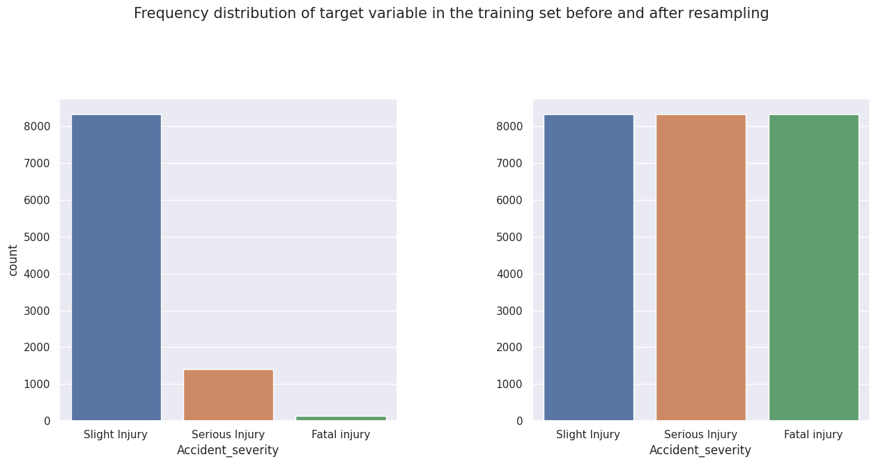
Before we proceed further, we encode the target variable using the following map:
Slight Injury\(\to 1\)Serious Injury\(\to 2\)Fatal injury\(\to 3\)
Feature Selection
To select the features to be used in the modeling phase, we employ chi-squared feature selection from the feature_selection module of scikit-learn library.
This method requires the input data not to contain any negative values. For this purpose, we have the following function which takes a DataFrame as input and relocates each column with negative values to make the resulting DataFrame consisting entirely of nonnegative values.
def spread_positivity(data):
    data_positive = data.copy(deep = True)
    for feature in data_positive.columns:
        if np.any(data_positive[feature] < 0) == True:
            min_ = data_positive[feature].min()
            data_positive[feature] = data_positive[feature] - min_
    return data_positive
The next function implements the chi-squared feature selection scheme. Note that the argument \(k\)
determines the number of columns to be retained before we proceed to the modeling phase. If it is a positive integer, then \(k\)
features with the highest SelectKBest scores are retained. If it is set as 'all', then all features are retained.
from sklearn.feature_selection import SelectKBest, chi2
def feature_selection_chi2(X_train, y_train, X_valid, X_test, k = 'all'):
    X_train = spread_positivity(X_train)
    X_valid = spread_positivity(X_valid)
    X_test = spread_positivity(X_test)
    fs = SelectKBest(score_func = chi2, k = k)
    fs.fit(X_train, y_train)
    cols = fs.get_support(indices = True)
    X_train_fs = X_train.iloc[:, cols]
    X_valid_fs = X_valid.iloc[:, cols]
    X_test_fs = X_test.iloc[:, cols]
    return X_train_fs, X_valid_fs, X_test_fs, fs
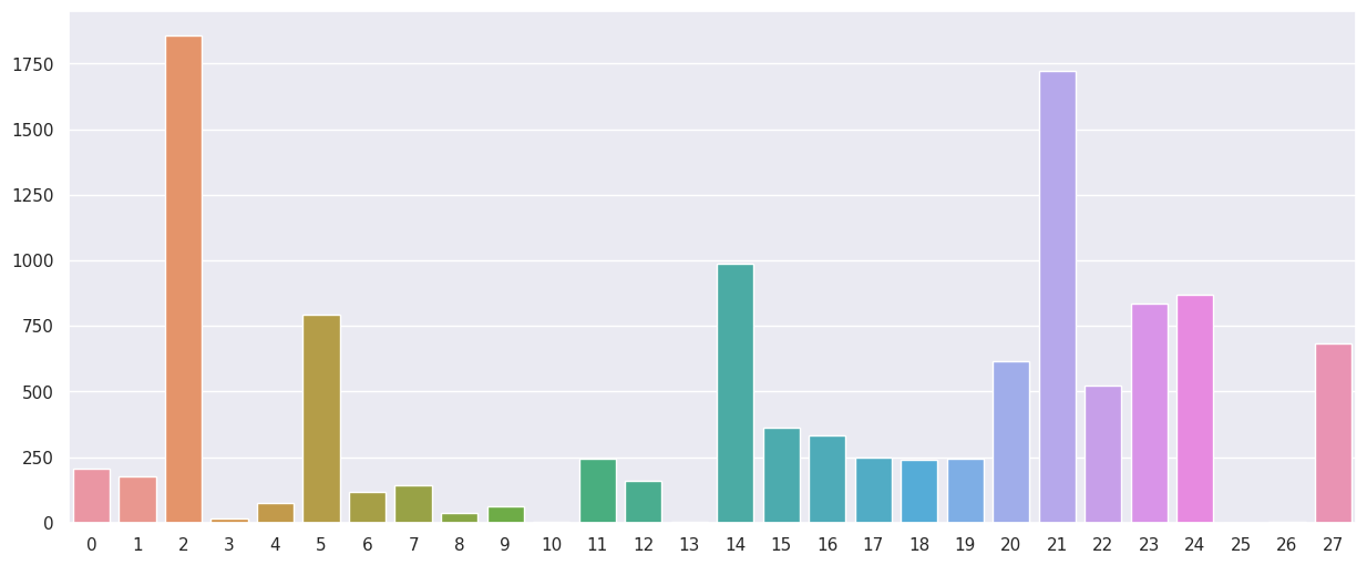
We retain all features by setting k = 'all' and plot the SelectKBest scores of the features (which are converted to positive integers).
○ Baseline Models
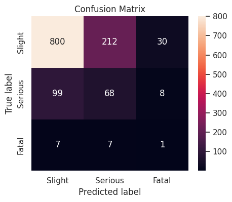
Decision Tree
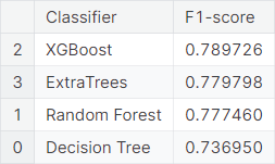
The decision Tree classifier with default hyperparameter values produces a weighted \(F_1\)-score of \(0.736950\) on the validation set.
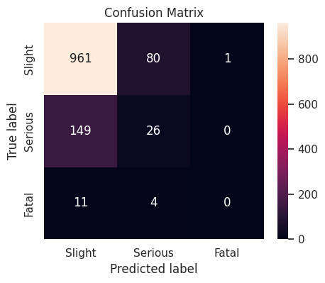
Random Forest
The random forest classifier with default hyperparameter values produces a weighted \(F_1\)-score of \(0.777460\) on the validation set.
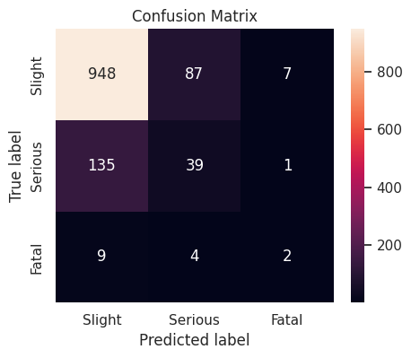
XGBoost
The XGBoost classifier with default hyperparameter values produces a weighted \(F_1\)-score of \(0.789726\) on the validation set.
ExtraTrees
The ExtraTrees classifier with default hyperparameter values produces a weighted \(F_1\)-score of \(0.779798\) on the validation set.

Summary of Baseline Models
The performance of the baseline models considered, ranked by the weighted \(F_1\)-score, is summarized below.
○ Hyperparameter Tuning
The baseline XGBoost classifier gives the highest validation weighted \(F_1\)-score. However, the ExtraTrees classifier and the random forest classifier are not far behind either. So, we employ the traditional grid search technique for hyperparameter tuning on these three classifiers.
Specifically, we use \(3\)-fold cross-validation on the training set for each of the hyperparameter grid points to choose the best one in terms of the cross-validation weighted \(F_1\)-score. We then proceed to check how the chosen model performs on the test set.
Tuning of Random Forest
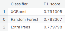
The random forest classifier with following hyperparameter values produces a cross-validation weighted \(F_1\)-score of \(0.925659\), and a weighted \(F_1\)-score of \(0.782367\) on the validation set.
Best hyperparameter values: {
  'class_weight': 'balanced',
  'criterion': 'entropy',
  'max_depth': None,
  'max_features': 'log2',
  'n_estimators': 200
}
Tuning of XGBoost
The XGBoost classifier with following hyperparameter values produces a cross-validation weighted \(F_1\)-score of \(0.937394\), and a weighted \(F_1\)-score of \(0.791005\) on the validation set.
Best hyperparameter values: {
    'gamma': 0,
    'learning_rate': 0.1,
    'max_depth': 10,
    'min_child_weight': 1,
    'n_estimators': 500,
    'reg_alpha': 0,
    'reg_lambda': 2,
    'subsample': 0.8
}

Tuning of ExtraTrees
The ExtraTrees classifier with following hyperparameter values produces a cross-validation weighted \(F_1\)-score of \(0.942512\), and a weighted \(F_1\)-score of \(0.779798\) on the validation set.
Best hyperparameter values: {
    'ccp_alpha': 0.0,
    'class_weight': 'balanced',
    'criterion': 'gini',
    'max_depth': None,
    'min_samples_split': 2
}

Summary of Tuned Models
The performance of the hyperparameter-tuned models on the validation set, ranked by the weighted \(F_1\)-score, is summarized below.
○ Prediction and Evaluation
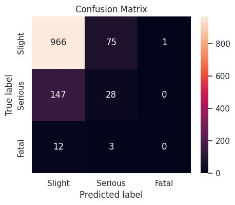
The tuned XGBoost model performs best on the validation set in terms of weighted \(F_1\)-score. We fit this model on the training set and predict on the test set, obtaining a weighted \(F_1\)-score of \(0.795060\).

○ Acknowledgements
- Bedane, Tarikwa Tesfa \((2020)\), “Road Traffic Accident Dataset of Addis Ababa City”, Mendeley Data, V\(1\), doi: 10.17632/xytv86278f.1
- Road Traffic Accidents dataset by Saurabh Shahane
○ References
- Correlation
- Cross-validation
- Curse of dimensionality
- Data preprocessing
- Decision tree
- Exploratory data analysis
- ExtraTrees
- Feature selection
- \(F\)-score
- Grid search
- Harmonic mean
- Heatmap
- Hyperparameter
- Hyperparameter optimization
- Min-max normalization
- Multiclass classification
- One-hot
- Outlier
- Precision
- Random forest
- Recall
- scikit-learn
- Synthetic minority over-sampling technique
- Test set
- Training set
- Train-test split
- Validation set
- XGBoost