Patient Survival Prediction
Deriving a quick understanding of the overall health of a patient is of paramount importance in emergency healthcare situations. Often, this understanding is hindered for many different reasons. In particular, the intensive care units in hospitals often lack a verified medical history of the incoming patients. The knowledge of medical records indicates the survival odds of a patient to a great extent. In this project, we predict whether a patient will survive or not based on various relevant medical information.
○ Contents
- Overview
- Introduction
- Exploratory Data Analysis
- Train-Test Split
- Data Preprocessing
- Baseline Neural Network
- Hyperparameter Tuning
- Prediction and Evaluation
- Acknowledgements
- References
○ Overview
- Information about the medical records of a patient plays a crucial role in determining his or her survival odds to a substantial extent.
- In this project, we aim to predict survival of a patient, which is a binary variable, based on the relevant medical records.
- A detailed exploratory data analysis on the dataset is carried out.
- We use the insights obtained from EDA in the data preprocessing stages, which consists of missing data imputation, categorical data encoding, and feature scaling.
- We build a neural network and tune it to predict survival of a patient.
- The final model obtains a test accuracy of \(0.923513\).
○ Introduction
Deriving a quick understanding of the overall health of a patient is of paramount importance in emergency healthcare situations. Often this understanding is hindered for many different reasons.
A patient in distress or in an unresponsive state may not be able to inform the healthcare professionals about chronic conditions such as heart disease, diabetes or other injuries. In particular, the intensive care units in the hospitals often lack verified medical history of the incoming patients. Also, when a patient shifts from one medical support provider to another, the clinical records of the patient may take days to transfer, which delays the treatment process. The pandemic situations present the health workers with these issues at a much larger scale as the hospitals may get overloaded with patients in severe conditions.
Knowledge about the medical records of a patient is crucial in the treatment process. It also plays a significant role in determining his or her survival odds to a substantial extent. We aim to build a predictive model of survival based on the relevant medical records.
Data
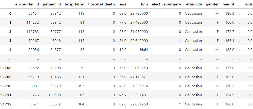
The dataset contains \(91713\) observations, each with \(186\) attributes.
Project Objective
The medical records of a patient play a significant role in determining his or her survival odds to a substantial extent. In this project, the objective is to predict whether a patient will survive or not, based on various relevant medical information. Thus, it is a binary classification problem.
Evaluation Metric
Let us denote
- TP: Number of true positives
- TN: Number of true negatives
- FP: Number of false positives
- FN: Number of false negatives
The accuracy metric is defined as the proportion of correct predictions. In terms of the notations mentioned above, it is given as
In this project, we use this metric to evaluate the models.
○ Exploratory Data Analysis
Understanding Features
This DataFrame describes the attributes in the original dataset through a six-point summary:
- Category
- Variable Name
- Unit of Measure
- Data Type
- Description
- Example

Dataset Synopsis
- Number of observations: \(91713\)
- Number of columns: \(186\)
- Number of integer columns: \(8\)
- Number of float columns: \(170\)
- Number of object columns: \(8\)
- Number of duplicate observations: \(0\)
- Number of duplicate columns: \(3\)
- Constant column:
readmission_status - Number of columns with missing values: \(175\)
- Columns with over \(90\%\)
missing values:
h1_bilirubin_max,h1_bilirubin_min,h1_lactate_min,h1_lactate_max,h1_albumin_max
The column readmission_status has the same value for every single observation and hence does not contribute to the task of classifying the observations. Thus, we remove this column.
Univariate Analysis
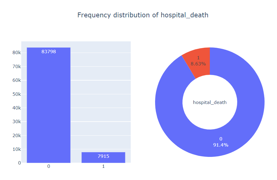
We begin by visualizing the frequency distribution of the target variable hospital_death, which is a binary variable indicating the survival status of a patient.
Next, we consider the predictor variables.
We observe that many of the columns are almost constant in the sense that the values in these columns are identical for most observations. More objectively, we say that a particular column is almost constant with respect to a threshold value \(p\)
if the relative frequency of the mode of the column is greater than \(p\).
The following function identifies the almost constant columns of an input DataFrame with respect to an input threshold value. If show = True, then it prints a series of these columns along with the relative frequency of the corresponding mode. Additionally, if return_list = True, then it returns a list of the almost constant columns.
def almost_constant(df, threshold = 0.9, show = True, return_list = True):
    rel_freq = []
    for col in df.columns:
        mode_rel_freq = max(df[col].value_counts(sort = True) / len(df[col]))
        if mode_rel_freq > threshold:
            rel_freq.append((col, mode_rel_freq))
    keys = [item[0] for item in rel_freq]
    values = [item[1] for item in rel_freq]
    series = pd.Series(data = values, index = keys).sort_values(ascending = False)
    if show == True:
        print(series.to_string())
    if return_list == True:
        return keys
We set the threshold value at \(0.9\) to find \(10\) almost constant features.
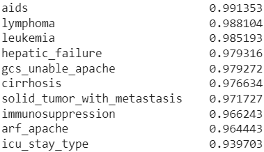
Among these features, icu_stay_type is an object variable, taking values admit, transfer and readmit, while the rest are binary float variables, taking values 0.0 and 1.0.
- Binary columns except
genderandhospital_death
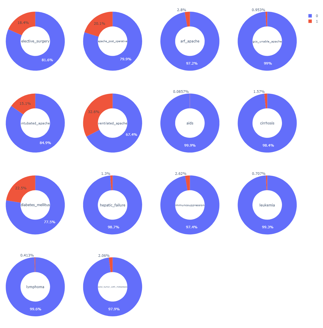
genderandicu_stay_type

- Columns with \(4\) to \(15\) distinct values

- Non-float columns with more than \(15\) distinct values
Four non-float columns, namely encounter_id, patient_id, hospital_id, and icu_id, have more than \(15\)
distinct values.

Among these, encounter_id and patient_id are unique for each observation, and hence do not contribute to the task of predicting the target variable. For this reason, we drop these two columns.
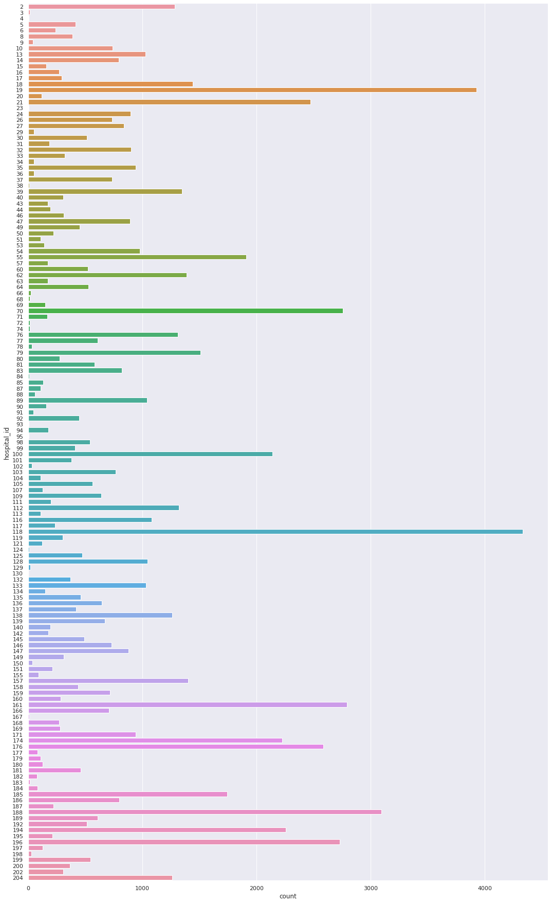
We present countplot for hospital_id.
Next, we present countplot for icu_id.

- Float columns with more than \(15\) distinct values
We visualize the distributions of the float columns with more than \(15\) distinct values.

Multivariate Analysis
- Relationships among the predictor variables
First, we consider the correlation structure among the numerical features. The color-coded correlation heatmap suggests that there are several pairs of features that are highly correlated. The image can be opened in a new tab and zoomed in for clarity.
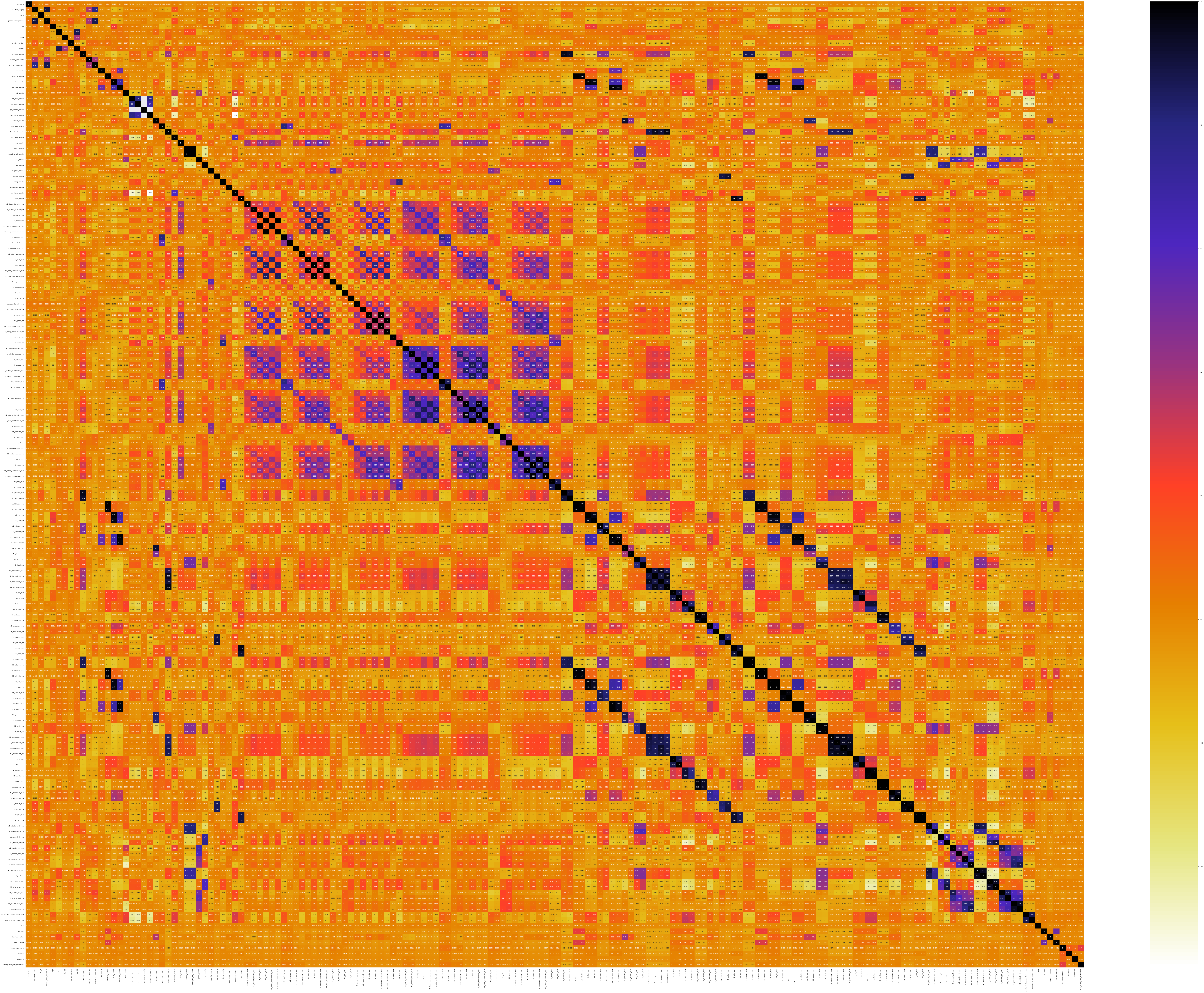
We identify the pairs of features with absolute correlation coefficient greater than \(0.9\) (i.e., correlation coefficient \(> 0.9\) or \(< -0.9\) ) and present them along with their correlation coefficient.

We observe that
- There are \(94\) pairs of numerical features with correlation coefficient over \(0.9\)
- There are no pair of numerical features with correlation coefficient below \(-0.9\)
- Three pairs of numerical features have correlation coefficient exactly equal to \(1\), i.e. there exists perfect linear relationship (with positive slope) between the variables in each of those pairs (this corresponds to the fact that there are \(3\) duplicate columns in the dataset)
- Relationships of the target variable with the predictor variables
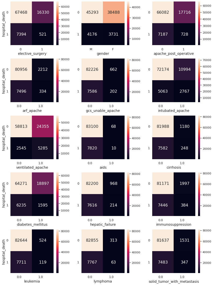
We present contingency tables for the target variable hospital_death and each binary feature in data.
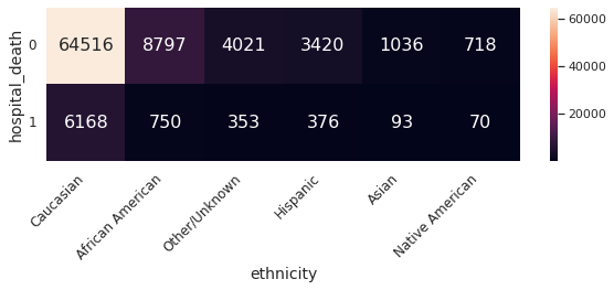
We present contingency tables for the target variable and each feature taking \(3\)
to \(15\)
distinct values. As an example, we show the contingency table for the target variable and ethnicity. For the complete output, see this notebook.
Next, we present kernel density estimate plot of numerical features, having more than \(15\) distinct values, for the two target classes.

○ Train-Test Split
We split the dataset into training set and test set in \(80:20\)
ratio using the train_test_split function.
The frequency distribution of the target variable in the training set and the test set is presented below.


○ Data Preprocessing
Missing Data Imputation
First, we check the count of missing values for the target variable.

Now, we move on to the predictor variables and identify the columns with more than \(50\%\) missing values in the training set.
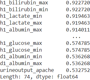
We drop the \(74\) features, which have over \(50\%\) values missing in the training dataset, from the subsequent analysis.
Proportional imputation: With the goal of keeping the feature distributions same before and after imputation, we impute the missing values in a column in such a way so that the proportions of the existing unique values in the column remain roughly same as those were prior to the imputation. The next function implements the idea.
def prop_imputer(data):
    data_prop = data.copy(deep = True)
    missing_cols = data_prop.isna().sum()[data_prop.isna().sum() != 0].index.tolist()
    for col in missing_cols:
        values_col = data_prop[col].value_counts(normalize = True).index.tolist()
        probabilities_col = data_prop[col].value_counts(normalize = True).values.tolist()
        data_prop[col] = data_prop[col].fillna(pd.Series(np.random.choice(values_col, p = probabilities_col, size = len(data))))
    return data_prop
We apply it on the training features and the test features.
Categorical Data Encoding
We present the categorical columns along with the respective number of unique values.

Categorical variables can be ordinal (ordered, e.g. very bad, bad, good, very good) or nominal (unordered, e.g. red, blue, yellow, green). We observe that all \(8\) categorical features are nominal in nature, i.e. there is no notion of order in their realized values.
The following function implements one-hot encoding to the selected columns (in an input list cols) of an input DataFrame data using the get_dummies function.
def one_hot_encoder(data, cols, drop_first = False):
    cols = [col for col in cols if col in data.columns]
    data_ohe = pd.get_dummies(data, columns = cols, drop_first = drop_first)
    return data_ohe
We encode the categorical columns of both training set and test set using this function.
For a categorical column with \(k\)
distinct values, the one-hot encoder produces \(k\)
new columns, one corresponding to each unique value. The original column is then dropped. As an example, we show the columns generated from the categorical column gender in the training set.
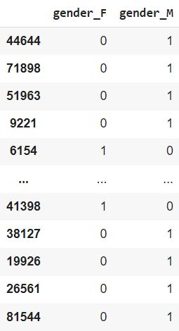
Observe that gender_F and gender_M are related by gender_F + gender_M = 1. Hence, we will lose no information by dropping one between these two columns. This can be done (for each feature) by setting drop_first = True.
The encoder now produces \(k-1\)
new columns for a categorical column with \(k\)
distinct values, as the first column is dropped. As before, the original column is also dropped. Under this scheme, we have only one column generated from the categorical column gender in the training set, with the first column gender_F being dropped.
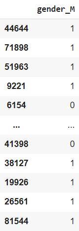
To have a column corresponding to nan values, if they are present in the original column, one must set the dummy_na parameter of the get_dummies function to be True. By default it is set as False.
Feature Scaling
It may be natural for one feature variable to have a greater impact on classification procedure than another. But often this is generated artificially by the difference of range of values that the features take. The unit of measurement in which the features are measured can be one a possible reason for such occurrence.
This necessitates the practitioner to scale the features appropriately before feeding the data to machine learning algorithms. For this purpose, the min-max normalization transforms the features in the following way:
The next function implements this using the MinMaxScaler class from the scikit-learn library. To keep the transformation the same, we use the minimum and maximum values of the training columns only for both DataFrames. Using the minimum and maximum values of the test columns for both sets would have led to data leakage.
Specifically, we use \(\min{\left(x\right)}\) and \(\max{\left(x\right)}\) for a particular feature from the training set to rescale the feature for both the training set and the test set.
def scaler(X_train, X_test):
    scaling = MinMaxScaler().fit(X_train)
    X_train_scaled = scaling.transform(X_train)
    X_test_scaled = scaling.transform(X_test)
    return X_train_scaled, X_test_scaled
○ Baseline Neural Network
Model Creation
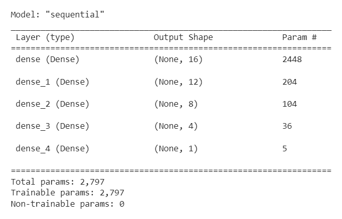
We begin by adding dense layers, with appropriate number of units and activation function, to a sequential model.
model = Sequential()
model.add(Dense(16, input_dim = len(X_train.columns), activation = 'relu'))
model.add(Dense(12, activation = 'relu'))
model.add(Dense(8, activation = 'relu'))
model.add(Dense(4, activation = 'relu'))
model.add(Dense(1, activation = 'sigmoid'))
A summary of the model is given below.
Model Compilation
We compile the model with binary cross-entropy loss and Adam optimizer. The model is evaluated with the accuracy metric during training and testing.
model.compile(
    loss = 'binary_crossentropy',
    optimizer = 'adam',
    metrics = ['accuracy']
)
Model Fitting
We fit the model for \(100\) epochs on the entirety of the training set, with \(64\) samples in each batch of training.
history = model.fit(
    X_train, y_train,
    validation_data = (X_test, y_test), # check the note below
    epochs = 100,
    batch_size = 64
)
Note: Feeding the test observations into validation_data can be dangerous in usual practice, as it risks data leakage. However, in this work, it does not happen, as we use the test set information neither in the training process nor in selecting any other parameters, such as the best epoch.
In fact, we take the model instance after the final epoch as the baseline, irrespective of the behavior of the model loss along the way. The purpose of using the test observations here is only to visualize how the model performance on the test set evolves through the epochs.
During the hyperparameter tuning process, though, the validation data become relevant in selecting the best model instance (through the choice of the best epoch), which will be used to predict and evaluate on the test set. Hence, using test observations in validation_data will invite data leakage. So, in the next section, we shall use a chunk of the training set through the validation_split parameter.
We present the loss and the accuracy scores for both the training set and the test set in the last fifteen epochs.
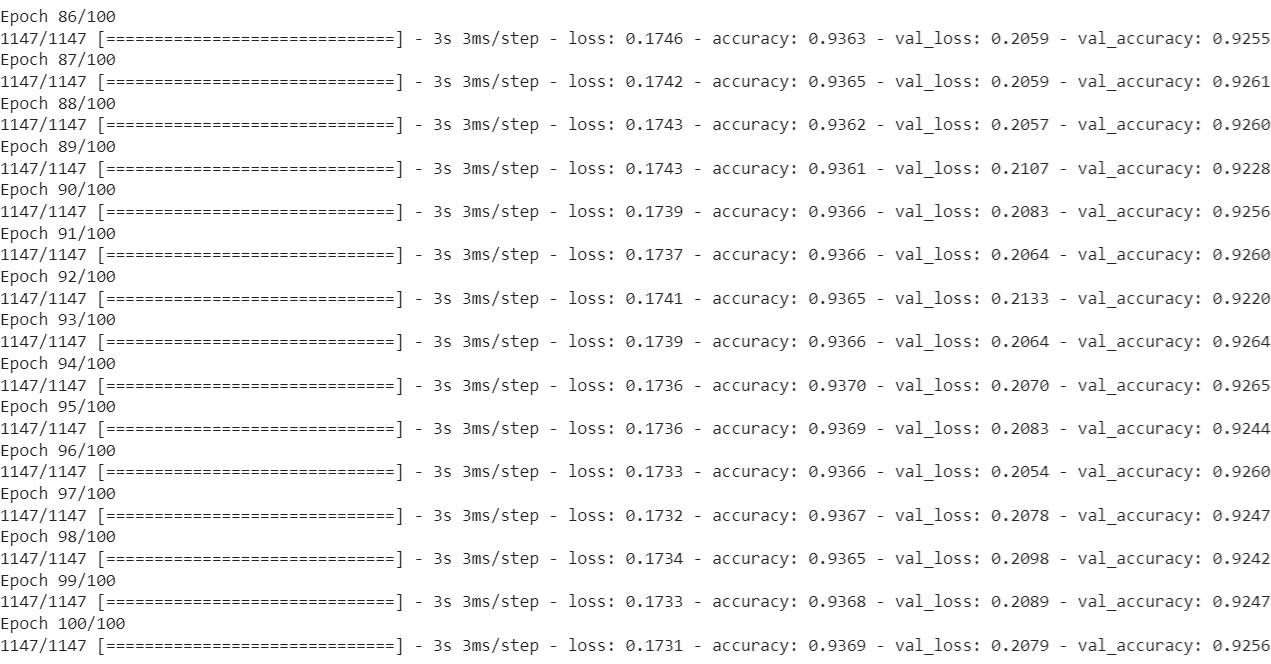
We plot the model loss (binary cross-entropy) for both the training set and the test set against the epochs.
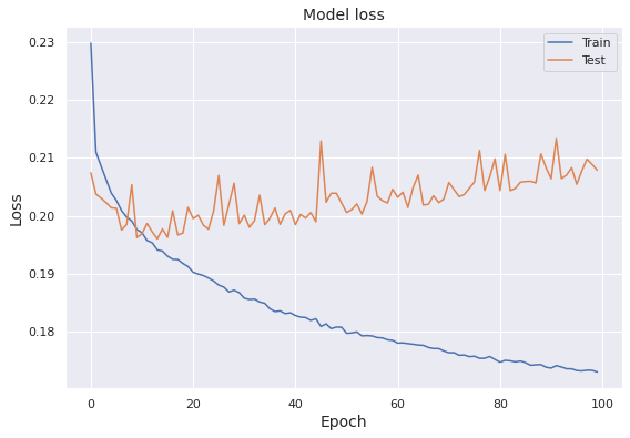
We note that, while the training loss expectedly declines over epochs, the test loss has a slow increasing trend after the initial decline. Next, we show how the training accuracy and the test accuracy evolve over epochs.
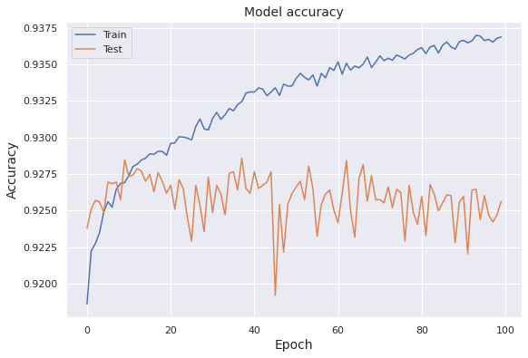
The result syncs with the behavior of the training loss and the test loss, as the training accuracy steadily increases over epochs and the test accuracy shows a slow declining trend.
Model Evaluation
Now, we use the fitted model to predict on the test set and convert the predicted class probabilities to class labels.
The baseline neural network obtains a test accuracy of \(0.925639\).
○ Hyperparameter Tuning
In this project, we tune the number of units in the first dense layer and the learning rate for the optimizer using the KerasTuner library.
Model Builder
The next function builds a model, with specified set of values for the hyperparameters to be optimized.
def model_builder(ht):
    model = Sequential()
    model.add(keras.layers.Flatten(input_shape = (X_train.shape[1],)))

    ht_units = ht.Int('units', min_value = 32, max_value = 512, step = 32)
    model.add(keras.layers.Dense(units = ht_units, activation = 'relu'))
    model.add(keras.layers.Dense(12, activation = 'relu'))
    model.add(keras.layers.Dense(8, activation = 'relu'))
    model.add(keras.layers.Dense(4, activation = 'relu'))
    model.add(keras.layers.Dense(1, activation = 'sigmoid'))

    ht_learning_rate = ht.Choice('learning_rate', values = [0.01, 0.001, 0.0001])
    model.compile(
        loss = 'binary_crossentropy',
        optimizer = Adam(learning_rate = ht_learning_rate),
        metrics = ['accuracy']
    )

    return model
Keras Tuner
We now make the tuner using the Hyperband function, setting the objective as validation accuracy.
tuner = kt.Hyperband(
    model_builder,
    objective = 'val_accuracy',
    max_epochs = 10,
    factor = 3,
    directory = 'dir_1'
)
Early Stopping
We use the early stopping callback to monitor the validation loss and stop the training once it stops improving by a specified margin for a specified number of epochs.
stop_early = tf.keras.callbacks.EarlyStopping(
    monitor = 'val_loss',
    patience = 5
)
Tuner Search
We implement the tuner using the search function, where we set the number of epochs to \(50\)
and incorporate the early stopping callback.
tuner.search(
    X_train, y_train,
    epochs = 50,
    validation_split = 0.2,
    callbacks = [stop_early]
)
The hyperparameter optimization results are summarized as follows.

Tuned Model Fitting
We build the model with optimal hyperparameter values and fit it on the training set. Specifically, we set aside \(20\%\)
training observations as validation data through the argument validation_split. We train the model on the rest of the training observations and evaluate it on the validation data. Observing the initially decreasing and then slowly increasing pattern of validation loss in the baseline model, we lower the number of epochs to \(50\).
best_hparams = tuner.get_best_hyperparameters(num_trials = 1)[0]
model = tuner.hypermodel.build(best_hparams)
history = model.fit(X_train, y_train, epochs = 50, validation_split = 0.2)
We present the loss and the accuracy scores for both the training set (except the chunk of \(20\%\) training observations set aside as validation set) and the validation set in an interval of fifteen epochs, highlighting the one giving the highest validation accuracy.
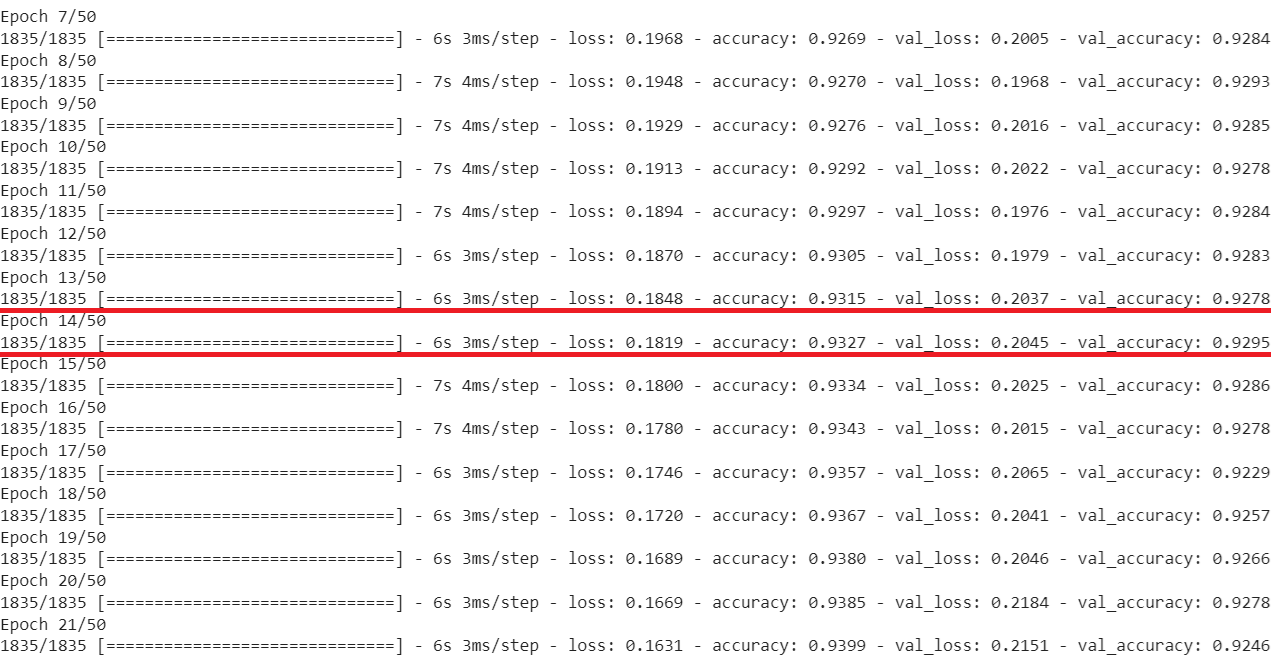
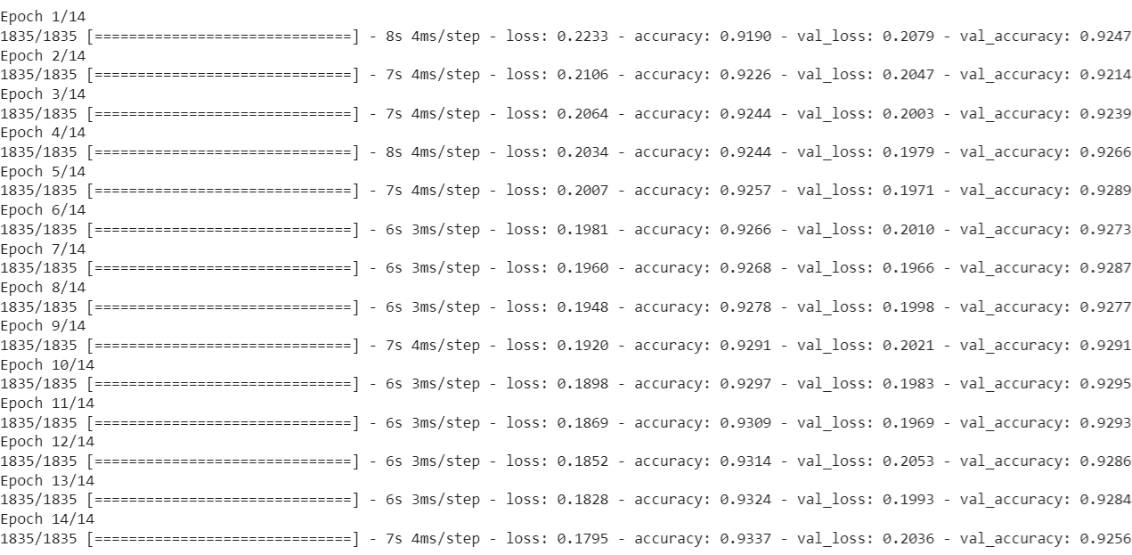
We retrieve the epoch producing the highest validation accuracy and re-instantiate the model with the optimal hyperparameter values.
val_accuracy_optimal = history.history['val_accuracy']
best_epoch = val_accuracy_optimal.index(max(val_accuracy_optimal)) + 1
model_tuned = tuner.hypermodel.build(best_hparams)
We re-train the model on the training set after setting aside \(20\%\)
of the training observations to form the validation set, with the number of epochs set to best_epoch.
model_tuned.fit(
    X_train, y_train,
    epochs = best_epoch,
    validation_split = 0.2
)
Note that the final epoch does not necessarily produce the highest validation accuracy.
○ Prediction and Evaluation
We use the tuned model to predict on the test set and convert the predicted class probabilities to class labels.
The tuned model obtains a test accuracy of \(0.923513\). While the overall performance decreases slightly, it is observed that the performance on the critical positive class improves. See this notebook for more details.
○ Acknowledgements
○ References
- Accuracy
- Activation function
- Adam optimizer
- Artificial neuron
- Binary classification
- Binary cross-entropy
- Binary variable
- Callback
- Categorical data encoding
- Correlation
- Correlation coefficient
- Data leakage
- Data preprocessing
- Dense layer
- Early stopping
- Exploratory data analysis
- Feature scaling
- Hyperparameter optimization
- KerasTuner
- Kernel density estimation
- Min-max normalization
- Missing data
- Imputation
- Mode
- Neural network
- One-hot
- Sequential model
- Test set
- Training set
- Unit of measurement