Natural Language Processing with Disaster Tweets
Disaster-related tweets have the potential to alert relevant authorities early on so that they can take action to reduce damage and possibly save lives. In this project, we attempt to predict whether a given tweet indicates a real disaster or not. We take a number of text normalization processes into consideration. For text representation, we experiment with the bag of words model (count vectorizer), TF-IDF vectorizer, and word2vec embedding. For each approach, we consider several binary classifiers and compare their performances through cross-validation.
○ Contents
- Overview
- Introduction
- Exploratory Data Analysis
- Text Normalization
- Bag of n-gram Model
- TF-IDF Model
- Word2Vec Model
- Conclusion
- Acknowledgements
- References
○ Overview
- Disaster-related tweets have the potential to alert relevant authorities early on so that they can take action to reduce damage and possibly save lives.
- In this project, we attempt to predict whether a given tweet indicates a real disaster or not.
- A detailed exploratory data analysis on the dataset is carried out.
- We consider a number of text normalization processes, namely conversion to lowercase, removal of whitespaces, removal of punctuations, removal of unicode characters (including HTML tags, emojis, and URLs starting with http), substitution of acronyms, substitution of contractions, removal of stop words, spelling correction, stemming, lemmatization, discardment of non-alphabetic words, and retention of relevant parts of speech.
- We implement bag of words text representation and extend the analysis to bag of bigrams as well as a mixture representation incorporating both words and bigrams.
- Next, we implement TF-IDF text representation. Similar to the previous setup, we carry out unigram, bigram, and mixture analysis.
- Finally, we use word2vec embedding for text representation.
- For each text representation setup, we apply a number of classifiers, namely logistic regression, \(k\)-nearest neighbors classifier, decision tree, support vector machine with radial basis function kernel, random forest, stochastic gradient descent, ridge classifier, XGBoost classifier, and AdaBoost classifier, and compare their performances in terms of the average \(F_1\)-score obtained from \(5\) repetitions of \(6\)-fold cross-validation.
- The support vector machine classifier with a radial basis function kernel acting on the embedded data obtained through the word2vec algorithm produces the best result in terms of the average \(F_1\)-score obtained from \(5\) repetitions of \(6\)-fold cross-validation. It achieves an average \(F_1\)-score of \(0.783204\).
○ Introduction
Twitter is one of the most active social media platform that many people use to share occurrence of incidents including disasters. For example, if a fire breaks out in a building, many people around the particular location are likely to tweet about the incident. These tweets can send early alerts not only to people in the neighbourhood to evacuate, but also to the appropriate authority to take measures to minimize the loss, potentially saving lives. Thus the tweets indicating real disasters can be utilized for emergency disaster management to remarkable effect. In this project, we attempt to predict whether a given tweet indicates a real disaster or not.
Data
Source: https://www.kaggle.com/c/nlp-getting-started/data
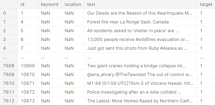
The training dataset contains information on \(7613\) tweets, each with a unique id, keyword (if available), location (if available), text and whether or not the tweet indicates a real disaster or not (expressed via a binary variable).
The test dataset contains information on \(3263\) tweets with the same features as above except the status of real disaster, which is to be predicted.
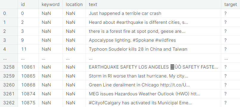
The features of the dataset are described below.
- id : A unique identifier corresponding to the tweet
- keyword : A highlighting word from the tweet
- location : The location from where the tweet is sent
- text: The textual content of the tweet
- target : A binary variable, which is \(0\) if the tweet does not indicate a real disaster and \(1\) if it does
Note that the features keyword and location may be blank for many tweets. Here we do not split the training set to hold a validation set out for evaluation purpose. Instead, we use repetition of \(k\)-fold cross-validation and take average performance to assess the models.
Project Objective
The objective of the project is to predict whether a particular tweet, of which the text (occasionally the keyword and the location as well) is provided, indicates a real disaster or not. Thus, it is a binary classification problem.
Evaluation Metric
Too much false positives, where a model detects disaster in a tweet that does not indicate any such occurrence, may be counterproductive and wasteful in terms of resources. Again, a false negative, where the model fails to detect a disaster from a tweet which actually indicates one, would delay disaster management and clearly costs too much. Let us denote
- TP: Number of true positives
- TN: Number of true negatives
- FP: Number of false positives
- FN: Number of false negatives
Precision and recall are universally accepted metrics to capture the performance of a model, when restricted respectively to the predicted positive class and the actual positive class. These are defined as
Observe that, in this problem, the class of tweets that indicate actual disasters (positive class) is more important than the class of tweets not indicating any disaster (negative class). Thus the goal is to build a model that attempts to minimize the proportion of false positives in the predicted positive class (maximize precision) and that of false negatives in the actual positive class (maximize recall), assigning equal emphasis on both. The \(F_1\)-score provides a balanced measuring stick by considering the harmonic mean of the above two matrics.
For its equal emphasis on both precision and recall, \(F_1\)-score is one of the most suitable metrics for evaluating the models in this project.
○ Exploratory Data Analysis
- Class frequency comparison
- Keywords associated with a tweet
- Location associated with a tweet
- Number of characters in a tweet
- Number of words in a tweet
- Average word-length in a tweet
- Number of URLs in a tweet
- Number of hashtags (#) in a tweet
- Number of mentions (@) in a tweet
- Punctuations in a tweet
Class frequency comparison
We begin by visualizing the class frequencies.
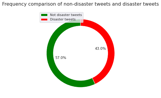
We observe that the training dataset is more or less balanced with respect to the target variable, which encodes whether or not a particular tweet indicates a disaster.
Next, we perform exploratory data analysis on a number of original and derived features in the training dataset.
Keywords associated with a tweet
Note: A lot of keywords contain two words joined by %20, which is the URL-encoding of the space character.
We visualize the top keywords, as per total count, for each class.
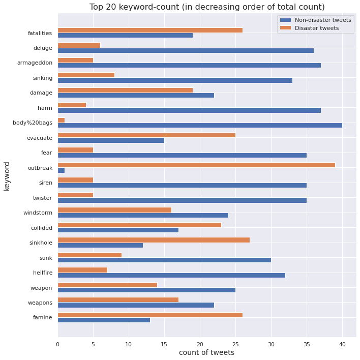
Since the sizes of the two classes are unequal, we cannot directly compare the count of a keyword in non-disaster tweets with the same in disaster tweets. To make a valid comparison, we must scale these counts by respective class sizes to obtain proportions of a keyword in non-disaster tweets and disaster tweets.
In particular, the absolute difference between these two quantities can be considered a measure of the ability of a keyword to discriminate between non-disaster tweets and disaster tweets. For instance, if the absolute difference is close to \(0\), then we cannot infer anything about the status of the tweet based on the keyword alone. On the other hand, a high value indicates that the keyword contributes significantly towards classifying the tweet into a particular class.
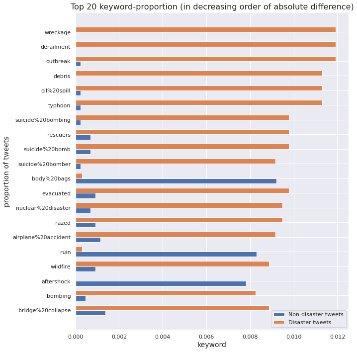
We investigate the \(5\) keywords with least absolute difference between proportion in non-disaster tweets and proportion in disaster tweets. Surprisingly, the keywords turn out to be bomb, weapons, landslide, flood, and disaster. These are usually associated with occurances of disasters. Although these words are used in non-disastrous contexts, for example landslide victory in an election or flood of joyful tears etc., it is still surprising for these to qualify as keywords in the non-disaster tweets.
Location associated with a tweet
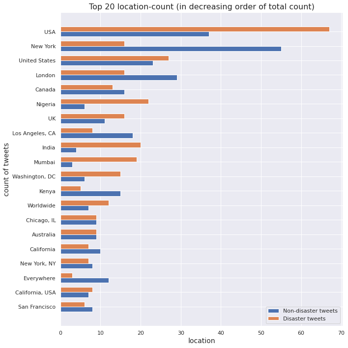
We visualize the top locations, as per total count, for each class.
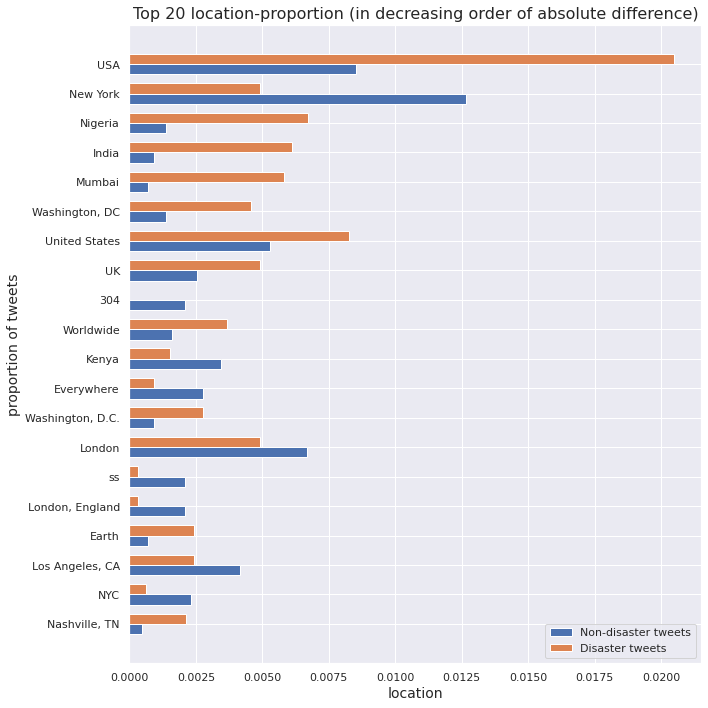
As in the case of keywords, we scale location counts by respective class sizes to obtain proportions of a location in non-disaster tweets and disaster tweets.
Number of characters in a tweet
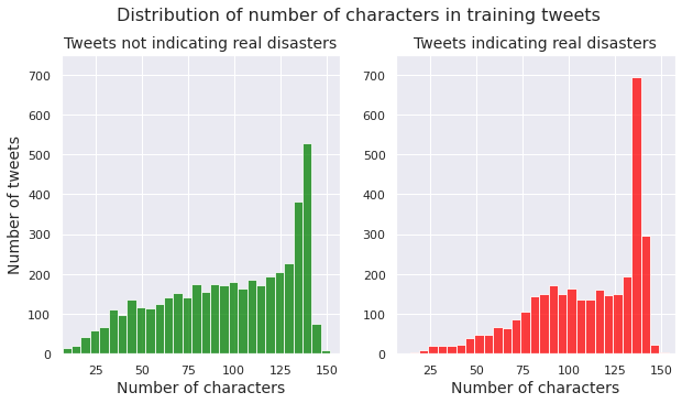
We examine the distribution of number of characters per tweet for both the class of non-disaster tweets and the class of disaster tweets.
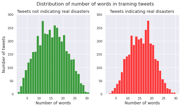
Number of words in a tweet
We examine the distribution of number of words per tweet for both the class of non-disaster tweets and the class of disaster tweets.
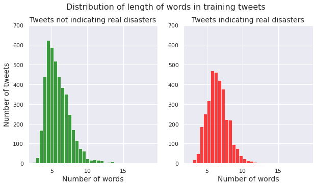
Average word-length in a tweet
Next we analyze the distribution of average word-length in tweets for both the class of non-disaster tweets and the class of disaster tweets.
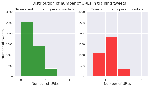
Number of URLs in a tweet
We examine the distribution of number of URLs per tweet for both the class of non-disaster tweets and the class of disaster tweets.
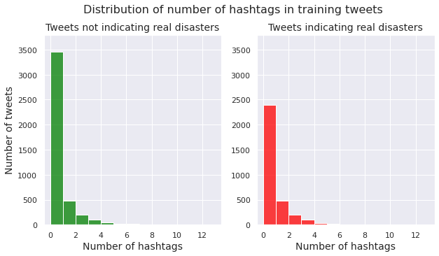
Number of hashtags (#) in a tweet
We examine the distribution of number of hashtags per tweet for both the class of non-disaster tweets and the class of disaster tweets.
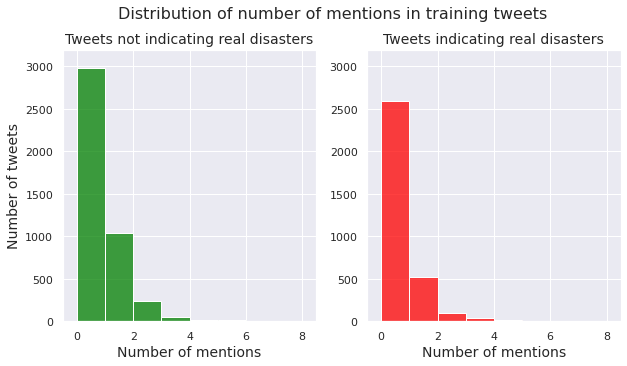
Number of mentions (@) in a tweet
We examine the distribution of number of mentions per tweet for both the class of non-disaster tweets and the class of disaster tweets.
Punctuations in a tweet
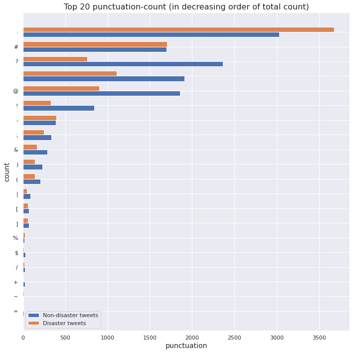
We visualize the top punctuations, as per total count, for each class.
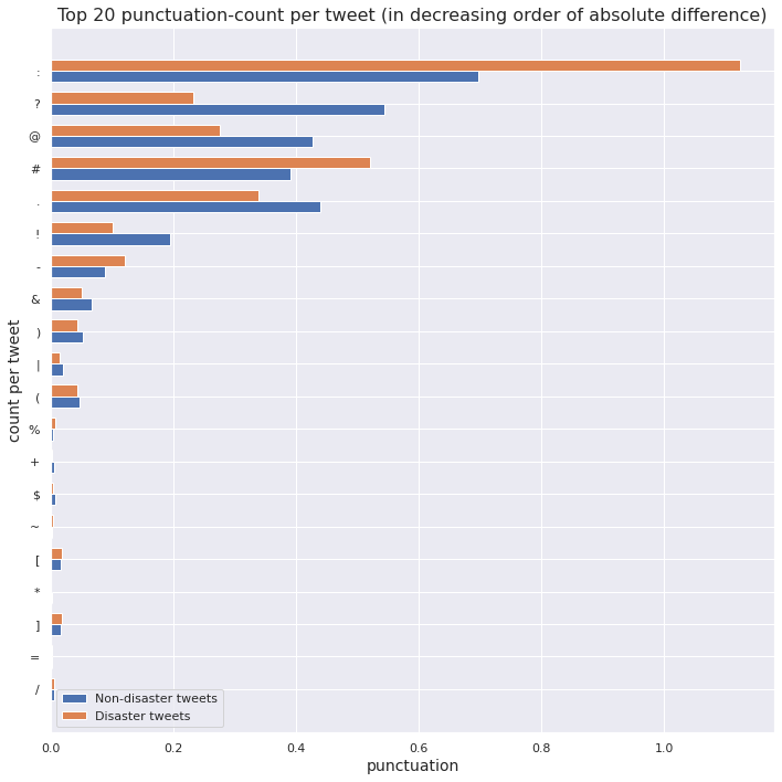
We scale punctuation counts by respective class sizes to obtain proportions of a punctuation in non-disaster tweets and disaster tweets.
Observations:
keywordfor \(99.2\%\) training tweets isNaN.- The \(5\) keywords with least absolute difference between their respective proportions in non-disaster tweets and disaster tweets are bomb, weapons, landslide, flood, disaster. These are usually associated with occurances of disasters. Although these words are used in non-disastrous contexts, for example landslide victory is an election or flood of joyful tears etc, it is still surprising for these to qualify as keywords in the non-disaster tweets.
locationfor \(66.7\%\) training tweets isNaN.- The distribution of most of the derived features are similar in case of disaster tweets (positive class) and non-disaster tweets (negative class).
Note: In the visualizations of class wise comparison of most features, including keyword and location, we produce only a few observations of the feature of interest due to the large number of distinct textual value taken by these features. The selection of these observations are done by considering certain attributes such as total count and choosing the top observations according to that attribute.
○ Text Normalization
- Conversion to lowercase
- Removal of whitespaces
- Removal of punctuations
- Removal of unicode characters
- Substitution of acronyms
- Substitution of contractions
- Removal of stop words
- Spelling correction
- Stemming and lemmatization
- Discardment of non-alphabetic words
- Retention of relevant parts of speech
- Integration of the processes
- Implementation of text normalization
Text normalization is the process of transforming text into a single canonical form that it might not have had before. We consider the following text normalization processes.
Conversion to lowercase
We convert all alphabetical characters of the tweets to lowercase so that the models do not differentiate identical words due to case-sensitivity. For example, without the normalization, Sun and sun would have been treated as two different words, which is not useful in the present context.
def convert_to_lowercase(text):
    return text.lower()
Removal of whitespaces
We remove the unnecessary empty spaces from the tweets.
def remove_whitespace(text):
    return text.strip()
Removal of punctuations
Mostly the punctuations do not play any role in predicting whether a particular tweet indicate disaster or not. Thus we prevent them from contaminating the classification procedures by removing them from the tweets. However, we keep apostrophe since most of the contractions contain this punctuation and will be automatically taken care of once we convert the contractions.
def remove_punctuation(text):
    punct_str = string.punctuation
    punct_str = punct_str.replace("'", "") # discarding apostrophe from the string to keep the contractions intact
    return text.translate(str.maketrans("", "", punct_str))
Removal of unicode characters
The training tweets are typically sprinkled with emojis, URLs, and other symbols that do not contribute meaningfully to our analysis, but instead create noise in the learning procedure. Some of these symbols are unique, while the rest usually translate into unicode strings. We remove these irrelevant characters from the data. We make use of the re module, which provides regular expression matching operations.
First we remove the HTML tags.
def remove_html(text):
    html = re.compile(r'<.*?>')
    return html.sub(r'', text)
Next, we remove the emojis.
def remove_emoji(text):
    emoji_pattern = re.compile(
        "["
        u"\U0001F600-\U0001F64F"  # emoticons
        u"\U0001F300-\U0001F5FF"  # symbols & pictographs
        u"\U0001F680-\U0001F6FF"  # transport & map symbols
        u"\U0001F1E0-\U0001F1FF"  # flags (iOS)
        u"\U00002702-\U000027B0"
        u"\U000024C2-\U0001F251"
        "]+", flags=re.UNICODE
    )
    return emoji_pattern.sub(r'', text)
We also remove URLs starting with http.
def remove_http(text):
    http = "https?://\S+|www\.\S+" # matching strings beginning with http (but not just "http")
    pattern = r"({})".format(http) # creating pattern
    return re.sub(pattern, "", text)
Substitution of acronyms
Acronyms are shortened forms of phrases, generally found in informal writings such as personal messages. Examples:
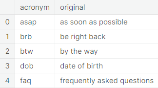
These time and effort-saving acronyms have received almost universal acceptance in social media platforms including twitter. For the sake of proper modeling, we convert the acronyms, appearing in the tweets, back to their respective original forms. For this purpose, we have compiled an extensive list of English acronyms, which can be found in the file:
english_acronyms_lowercase.json
Note that the file only considers acronyms in lowercase, i.e. it assumes that the textual data have already been transformed to lowercase before substituting the acronyms. For example, the process will convert fyi to for your information but will leave Fyi unchanged.
acronyms_url = 'https://raw.githubusercontent.com/sugatagh/E-commerce-Text-Classification/main/JSON/english_acronyms.json'
acronyms_dict = pd.read_json(acronyms_url, typ = 'series')
acronyms_list = list(acronyms_dict.keys())
The following function converts the acronyms, included in the .json file, appearing in any given input text.
def convert_acronyms(text):
    words = []
    for word in regexp.tokenize(text):
        if word in acronyms_list:
            words = words + acronyms_dict[word].split()
        else:
            words = words + word.split()
    text_converted = " ".join(words)
    return text_converted
Substitution of contractions
A contraction is a shortened form of a word or a phrase, obtained by dropping one or more letters. Examples:
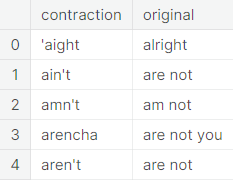
These are commonly used in everyday speech, written dialogue, informal writing and in situations where space is limited or costly, such as advertisements. Usually the missing letters are indicated by an apostrophe, but there are exceptions. We have compiled an extensive list of English contractions, which can be found here:
english_contractions_lowercase.json
Note that the file only considers contractions in lowercase, i.e. it assumes that the textual data have already been transformed to lowercase before substituting the contractions. For example, the process will convert i’ll to i shall but will leave I’ll unchanged.
contractions_url = 'https://raw.githubusercontent.com/sugatagh/E-commerce-Text-Classification/main/JSON/english_contractions.json'
contractions_dict = pd.read_json(contractions_url, typ = 'series')
contractions_list = list(contractions_dict.keys())
The following function converts the contractions, included in the .json file, appearing in any given input text.
def convert_contractions(text):
    words = []
    for word in regexp.tokenize(text):
        if word in contractions_list:
            words = words + contractions_dict[word].split()
        else:
            words = words + word.split()
    text_converted = " ".join(words)
    return text_converted
Removal of stop words
Several words, primarily pronouns, prepositions, modal verbs etc., are identified not to have much effect on the classification procedure. To get rid of the unwanted contamination effect, we remove these words. For this purpose, we use the stopwords module from NLTK. Some of these words are shown below.
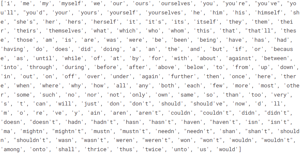
stops = stopwords.words("english") # stopwords
addstops = ["among", "onto", "shall", "thrice", "thus", "twice", "unto", "us", "would"] # additional stopwords
allstops = stops + addstops
def remove_stopwords(text):
    return " ".join([word for word in regexp.tokenize(text) if word not in allstops])
Spelling correction
The classification process cannot take misspellings into consideration and treats a word and its misspelt version as separate words. For this reason it is necessary to conduct spelling correction before feeding the data to the classification procedure. We use the pyspellchecker package for this purpose.
The next function corrects the misspelt words in a given input text.
spell = SpellChecker()
def pyspellchecker(text):
    word_list = regexp.tokenize(text)
    word_list_corrected = []
    for word in word_list:
        if word in spell.unknown(word_list):
            word_corrected = spell.correction(word)
            if word_corrected == None:
                word_list_corrected.append(word)
            else:
                word_list_corrected.append(word_corrected)
        else:
            word_list_corrected.append(word)
    text_corrected = " ".join(word_list_corrected)
    return text_corrected
Stemming and lemmatization
Stemming is the process of reducing the words to their root form or stem. It reduces related words to the same stem even if the stem is not a dictionary word. For example, the words introducing, introduced, introduction reduce to a common word introduce. However, the process often produces stems that are not actual words. The sentence Introducing lemmatization as an improvement over stemming becomes introduc lemmat as an improv over stem upon applying the stemming procedure. The stems introduc, lemmat and improv are not actual words. Here we use the Porter stemming algorithm.
The function to implement stemming is as follows.
stemmer = PorterStemmer()
def text_stemmer(text):
    text_stem = " ".join([stemmer.stem(word) for word in regexp.tokenize(text)])
    return text_stem
Lemmatization offers a more sophisticated approach by utilizing a corpus to match root forms of the words. Unlike stemming, it uses the context in which a word is being used. Upon applying lemmatization, the same sentence becomes introduce lemmatization as an improvement over stem. Here we use the spaCy lemmatizer.
We implement lemmatization through the following function.
spacy_lemmatizer = spacy.load("en_core_web_sm", disable = ['parser', 'ner'])
def text_lemmatizer(text):
    text_spacy = " ".join([token.lemma_ for token in spacy_lemmatizer(text)])
    return text_spacy
Discardment of non-alphabetic words
The non-alphabetic words are not numerous and create unnecessary diversions in the context of classifying tweets into non-disaster and disaster categories. Hence we discard these words.
def discard_non_alpha(text):
    word_list_non_alpha = [word for word in regexp.tokenize(text) if word.isalpha()]
    text_non_alpha = " ".join(word_list_non_alpha)
    return text_non_alpha
Retention of relevant parts of speech
The parts of speech provide a great tool to select a subset of words that are more likely to contribute in the classification procedure and discard the rest to avoid noise. The idea is to select a number of parts of speech that are important to the context of the problem. Then we partition the words in a given text into several subsets corresponding to each part of speech and keep only those subsets corresponding to the selected parts of speech. An alphabetical list of part-of-speech tags used in the Penn Treebank Project is given here.
def keep_pos(text):
    tokens = regexp.tokenize(text)
    tokens_tagged = nltk.pos_tag(tokens)
    keep_tags = ['NN', 'NNS', 'NNP', 'NNPS', 'FW', 'PRP', 'PRPS', 'RB', 'RBR', 'RBS', 'VB', 'VBD', 'VBG', 'VBN', 'VBP', 'VBZ', 'WDT', 'WP', 'WPS', 'WRB']
    keep_words = [x[0] for x in tokens_tagged if x[1] in keep_tags]
    return " ".join(keep_words)
Integration of the processes
We integrate the text normalization processes in appropriate order into one single function. Note that the spelling correction step takes a massive amount of time to run on large datasets and hence may be commented out for a quick implementation.
def text_normalizer(text):
    text = convert_to_lowercase(text)
    text = remove_whitespace(text)
    text = re.sub('\n' , '', text) # converting text to one line
    text = re.sub('\[.*?\]', '', text) # removing square brackets
    text = remove_http(text)
    text = remove_punctuation(text)
    text = remove_html(text)
    text = remove_emoji(text)
    text = convert_acronyms(text)
    text = convert_contractions(text)
    text = remove_stopwords(text)
    text = pyspellchecker(text)
    text = text_lemmatizer(text) # text = text_stemmer(text)
    text = discard_non_alpha(text)
    text = keep_pos(text)
    text = remove_additional_stopwords(text)
    return text
Implementation of text normalization
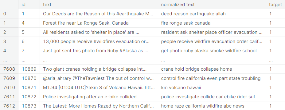
Next, we perform text normalization on the training tweets.
We perform the same on the test tweets.
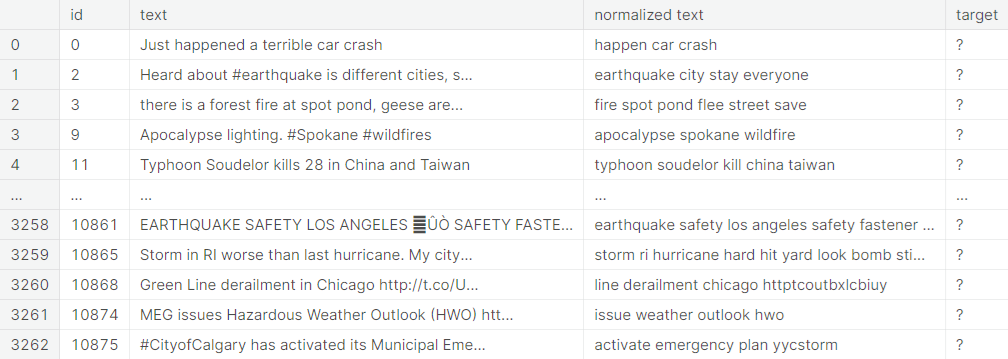
Here we consider only the normalized text as the predictor variable, leaving keyword and location out as they are missing for most tweets.
○ Bag of n-gram Model
In this section, we use the CountVectorizer class to convert the list of normalized texts to a matrix of token counts. We create an instance of this class by setting the ngram_range parameter, with the default choice being \((1, 1).\)
CountVec = CountVectorizer(ngram_range = (1, 1))
The parameter gives the lower and upper boundary of the range of \(n\)-values
corresponding to different word \(n\)-grams
to be extracted, i.e. all values of \(n\)
such that \(\text{min}_n \leq n \leq \text{max}_n\)
will be used. For example, an ngram_range of \((1, 1)\)
means only words, \((1, 2)\)
means words and bigrams, and \((2, 2)\)
means only bigrams.
Note that this implementation produces a sparse representation of the counts as compressed sparse row matrix. We shall need to convert it to DataFrame and then transform it back to the original format at a later stage in the modeling phase. For this purpose, we use the csr_matrix class from the sparse package of the SciPy library.
Bag of Words
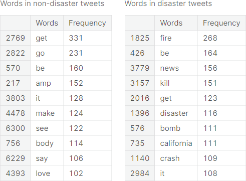
The bag of words model is a way of representing text data used in natural language processing. The model only considers multiplicity of the words and completely disregards the grammatical structure and ordering of the words.
The top \(10\) most frequent words, along with their respective frequencies, for both the positive class and the negative class, are documented in the following table.
We fit the bag of words model, treating each word as a feature. We observe the average \(F_1\)-score obtained from \(5\) repetitions of \(6\) -fold cross-validation using different classifiers.
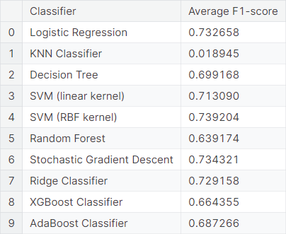
We observe that logistic regression, support vector machine (SVM) with radial basis function (RBF) kernel, stochastic gradient descent, and ridge classifier work well in this prediction scheme, compared to the other classifiers.
Next, we fit the same model, considering only the top \(10\%\) words as features. We observe the average \(F_1\)-score resulting from cross-validations using different classifiers.
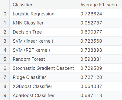
As in the model considering all words as features, logistic regression, SVM with RBF kernel, stochastic gradient descent and ridge classifier works well in the model considering only the top layer of words, compared to the other classifiers.
Bag of Bigrams
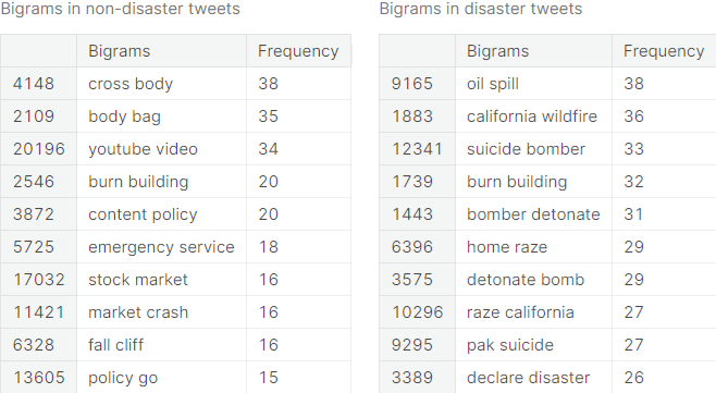
Next, we consider bag of bigrams (pair of consecutive words) model instead of bag of words model. The next function produces a DataFrame consisting of all possible bigrams from an input text corpus, along with their respective frequencies.
The top \(10\) most frequent bigrams, along with their respective frequencies, for both the positive class and the negative class, are documented in the following table.
We fit the bag of bigrams model, treating each bigram as a feature. We observe the average \(F_1\)-score obtained from \(5\) repetitions of \(6\)-fold cross-validation using different classifiers.
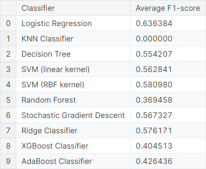
Next, we consider the same model with the top quarter \((25\%)\) of bigrams. We observe the average \(F_1\)-score obtained from \(5\) repetitions of \(6\)-fold cross-validation using different classifiers.
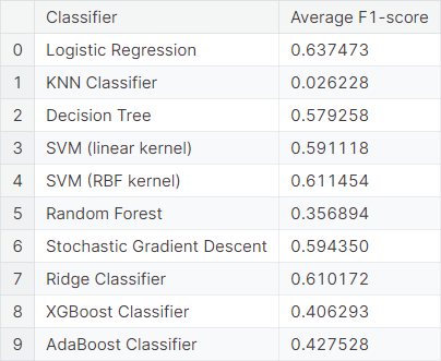
We observe that logistic regression, decision tree, SVM with RBF kernel, stochastic gradient descent and ridge classifier work moderately well for the bag of bigrams models, but not as well as the bag of words models.
Mixture Models
Now, we consider mixture models by considering both words as well as bigrams as features. We observe the average \(F_1\)-score obtained from \(5\) repetitions of \(6\)-fold cross-validation using different classifiers.
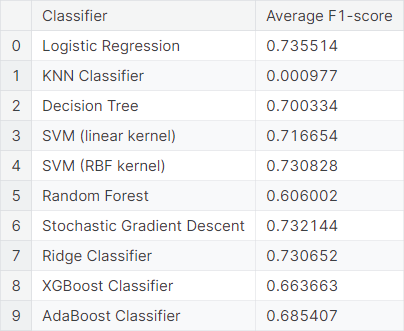
Next, we consider a mixture of features by considering top \(10\%\) words and top \(25\%\) bigrams. We observe the average \(F_1\)-score obtained from \(5\) repetitions of \(6\)-fold cross-validation using different classifiers.
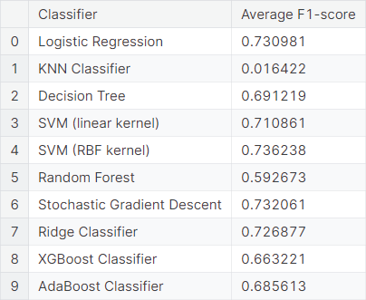
We observe that the performances under mixture models are more or less similar to those under bag of words models.
○ TF-IDF Model
In the context of information retrieval, TF-IDF (short for term frequency-inverse document frequency), is a numerical statistic that is intended to reflect how important a word is to a document in a collection or corpus. It is often used as a weighting factor in searches of information retrieval, text mining, and user modeling.
The TF-IDF value increases proportionally to the number of times a word appears in the document and is offset by the number of documents in the corpus that contain the word, which helps to adjust for the fact that some words appear more frequently in general.
Thus, the measure objectively evaluates how relevant a word is to a text in a collection of texts, taking into consideration that some words appear more frequently in general. For more details, check this note.
The TfidfVectorizer class converts a collection of raw documents to a matrix of TF-IDF features. Creating an instance of the class with the ngram_range parameter is similar to creating an instance of the CountVectorizer class, described in the previous section.
TfidfVec = TfidfVectorizer(ngram_range = (1, 1))
Bag of Words (TF-IDF)
First, we fit the TF-IDF model, treating each word as a feature. We observe the average \(F_1\)-score obtained from \(5\) repetitions of \(6\)-fold cross-validation using different classifiers.
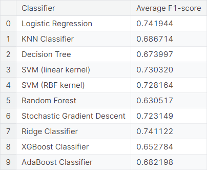
We observe that logistic regression, SVM with RBF kernel, stochastic gradient descent, and ridge classifier work well in this prediction scheme, compared to the other classifiers. In fact, logistic regression, the classifier returning the highest average \(F_1\)-score , has a slight improvement over the same model without TF-IDF implementation.
Next, we fit the same model, considering only the top \(10\%\) words as features. We observe the average \(F_1\)-score resulting from cross-validations using different classifiers.
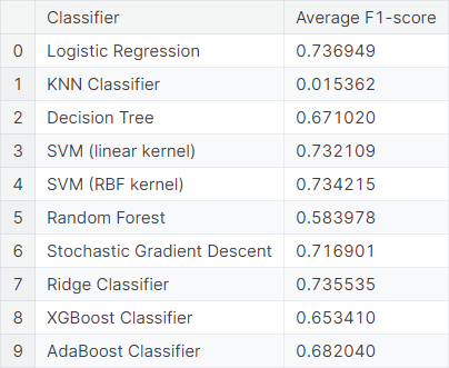
As in the model considering all words as features, logistic regression, SVM with RBF kernel, stochastic gradient descent and ridge classifier work well in the model considering only the top layer of words, compared to the other classifiers.
Bag of Bigrams (TF-IDF)
Next, we fit the TF-IDF model, treating each bigram as a feature. We observe the average \(F_1\)-score resulting from cross-validations using different classifiers.
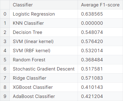
We fit the same model, considering only the top \(10\%\) bigrams as features. We observe the average \(F_1\)-score resulting from cross-validations using different classifiers.

Mixture Models (TF-IDF)
Next, we fit the TF-IDF model, considering both words as well as bigrams as features. We observe the average \(F_1\)-score resulting from cross-validations using different classifiers.

We fit the same model, considering only the top \(10\%\) words and the top \(10\%\) bigrams as features. We observe the average \(F_1\)-score resulting from cross-validations using different classifiers.
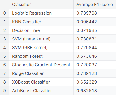
We observe that the results of the mixture models are more or less similar to that of the bag of words models. Also, the \(k\)-NN classifier works poorly in all the prediction schemes described above, except for the bag of words model treating each word as a feature.
○ Word2Vec Model
Roughly speaking, word embeddings are vector representations of a particular word. It has the ability to capture the context of a particular word in a document, as well as identify semantic and syntactic similarity and other contextual relations with other words in the document.
Word2Vec is a specific word-embedding technique that uses a neural network model to learn word associations from a fairly large corpus of text. After the model is trained, it can detect similarity of words, as well as recommend words to complete a partial sentence. True to its name, word2vec maps each distinct word to a vector, which is assigned in such a way that the level of semantic similarity between words are indicated by a simple mathematical operation on the vectors that the words are mapped to (for instance, the cosine similarity between the vectors).
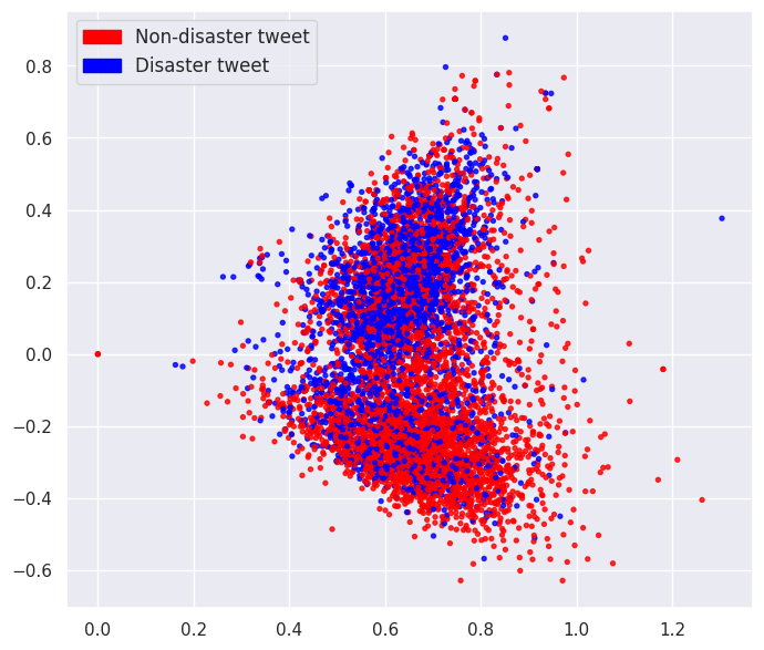
Here we use the raw text except for converting to lowercase and converting the contractions to their respective expanded forms. We do not use the other text normalization processes. Then, we tokenize the processed text and feed the tokens to the word2vec embedder. The embedded observations, color-coded by their class (non-disaster or disaster), are visualized in the following plot.
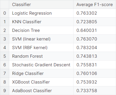
We convert the word2vec embeddings to a compressed sparse row matrix. Finally, we observe the average \(F_1\)-score obtained from \(5\) repetitions of \(6\)-fold cross-validation using different classifiers acting on the word embeddings obtained through the word2vec model.
○ Conclusion
We observe that the support vector machine classifier with a radial basis function kernel acting on the embedded data obtained through the word2vec algorithm produces the best result in terms of the average \(F_1\)-score obtained from \(5\) repetitions of \(6\)-fold cross-validation. It achieves an average \(F_1\)-score of \(0.783204\).
○ Acknowledgements
- Alphabetical list of part-of-speech tags used in the Penn Treebank Project
- List of English contractions
- Natural Language Processing with Disaster Tweets Dataset
○ References
- Acronym
- AdaBoost
- Bag of words
- Bigram
- Binary classification
- Canonical form
- Classifier
- Compressed sparse row
- Context
- Contraction
- Corpus
- Cosine similarity
- Cross-validation
- Decision tree
- Document
- Emoji
- Exploratory data analysis
- False negative
- False positive
- \(F\)-score
- Harmonic mean
- HTML
- HTTP
- Information retrieval
- Inverse document frequency
- \(k\)-nearest neighbors algorithm
- Lemmatization
- Lowercase
- Logistic regression
- Multiplicity
- Natural language processing
- Neural network
- NLTK
- Part of speech
- Precision
- Punctuation
- Random forest
- Regular expression
- Regular expression python module
- Recall
- Ridge classifier
- SciPy
- Semantic similarity
- SpaCy
- Sparse matrix
- Spelling
- Stemming
- Stochastic gradient descent
- Stop word
- Support vector machine
- Term frequency
- Test dataset
- Text mining
- Text normalization
- TF-IDF
- Training dataset
- Unicode character
- URL
- User modeling
- Vector
- Whitespace character
- Word embedding
- Word2Vec
- XGBoost