Higgs Boson Event Detection
In particle physics, events refer to the results just after a fundamental interaction took place between subatomic particles, occurring in a very short time span in a well-localized region of space. A background event is explained by the existing theories. On the other hand, a signal event indicates a process that cannot be described by previous observations and leads to the potential discovery of a new particle. In this project, we aim to predict if a given event is background or signal.
○ Contents
- Overview
- Introduction
- Exploratory Data Analysis
- Train-Test Split
- Data Preprocessing
- Feature Engineering
- Baseline Model
- Hyperparameter Tuning
- Prediction and Evaluation
- Acknowledgements
- References
○ Overview
- In particle physics, an event refers to the results just after a fundamental interaction took place between subatomic particles, occurring in a very short time span, at a well-localized region of space.
- A background event is explained by the existing theories and previous observations. On the other hand, a signal event indicates a process that cannot be described by previous observations and leads to the potential discovery of a new particle.
- In this project, we aim to predict if a given event is background or signal, based on the data provided in the Kaggle competition Higgs Boson Machine Learning Challenge.
- A detailed backdrop of the problem is given, and exploratory data analysis on the provided data is carried out.
- The observations obtained from EDA are used in the data preprocessing and feature engineering stages.
- We build a neural network and tune it to predict if a given event is background or signal.
- We employ the approximate median significance (AMS) metric to evaluate the models. The final model obtains a training AMS of \(2.500144\) and a test AMS of \(1.200022\). It achieves a training accuracy of \(0.827070\) and a test accuracy of \(0.824100\).
○ Introduction
Backstory
Particle accelerators enable physicists to explore the fundamental nature of matter by observing subatomic particles produced by high-energy collisions of particle beams. The experimental measurements from these collisions inevitably lack precision, which is where machine learning comes into picture. The research community typically relies on standardized machine learning software packages for the analysis of the data obtained from such experiments and spends a huge amount of effort towards improving statistical power by extracting features of significance, derived from the raw measurements.
The Higgs boson particle has been observed to decay into boson pairs. To establish that the Higgs field provides the interaction which gives mass to the fundamental fermions, it has to be demonstrated that the Higgs boson can decay into fermion pairs through direct decay modes. Subsequently, to seek evidence on the decay of Higgs boson into fermion pairs and to precisely measure their characteristics became one of the important lines of enquiry. Among the available modes, the most promising is the decay to a pair of tau leptons \(h \to \tau^+\tau^-\).
The first evidence of \(h \to \tau^+\tau^-\) decays was reported in \(2013\), based on the full set of proton-proton collision data recorded by the ATLAS experiment at the LHC during \(2011-2012\). Despite the consistency of the data with \(h \to \tau^+\tau^-\) decays, it could not be ensured that the statistical power exceeds the \(5\sigma\) threshold, which is the required standard for claims of discovery in high-energy physics community.
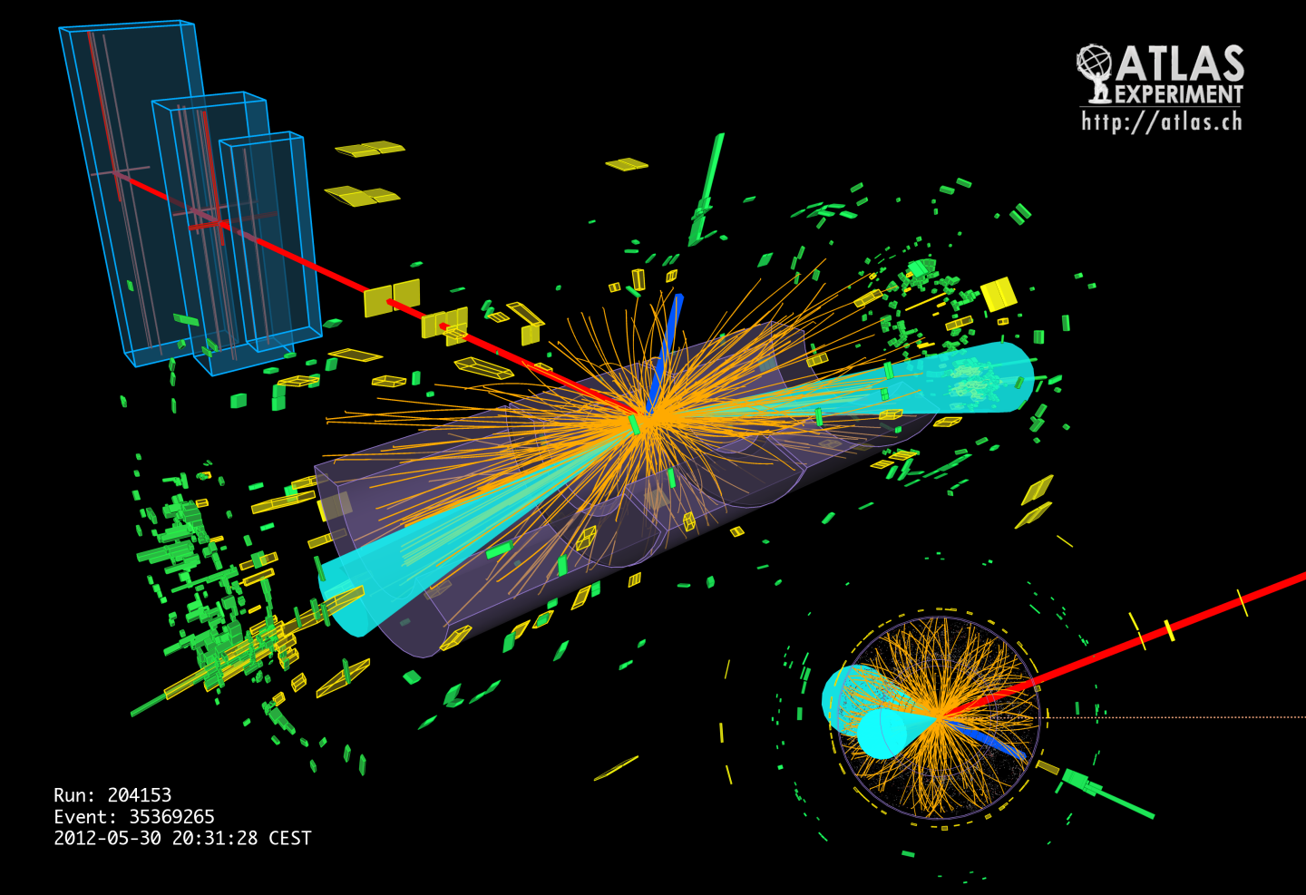
Higgs into fermions: Evidence of the Higgs boson decaying to fermions (image credit: CERN)
The aim of the offline analysis is to find a selection region in the feature space that produces a significant excess of events compared to what known background processes can explain. These are called signal events. Once the region has been fixed, a statistical test is applied to determine the significance of the excess. If the probability that the excess has been produced by background processes falls below a certain limit, it indicates the discovery of a new particle.
The broad goal is to improve the procedure that produces a selection region, i.e., the region (not necessarily connected) in the feature space that produces signal events.
Machine learning plays a major role in processing data resulting from experiments at particle colliders. The ML classifiers learn to distinguish between different types of collision events by training on simulated data from sophisticated Monte-Carlo programs. Shallow neural networks with single hidden layer are one of the primary techniques used for this analysis.
Efforts to increase statistical power tend to focus on developing new features for use with the existing ML classifiers. These high-level features are non-linear functions of the low-level measurements, derived using knowledge of the underlying physical processes.
The abundance of labeled simulation training data and the complex underlying structure make this an ideal application for deep learning. Large deep neural networks can simplify and improve the analysis of high-energy physics data by automatically learning high-level features from the data. In particular, they increase the statistical power of the analysis even without the help of manually derived high-level features.
Data
Source: https://www.kaggle.com/competitions/higgs-boson/data
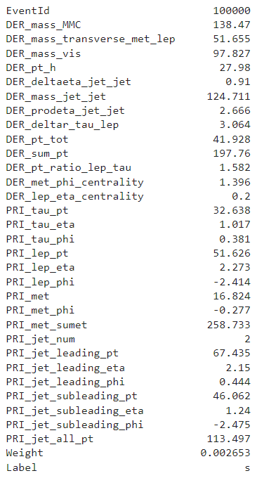
The training set contains \(250000\) observations of \(33\) columns.

An example of an observation from the training set is as follows.
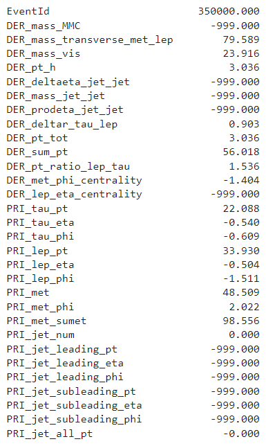
The test set contains \(550000\)
observations. It has all the columns of the training set except Label (signal or background) and Weight.

An observation from the test set typically looks like this.
Project Objective
The objective of the project is to classify an event produced in the particle accelerator as background or signal. As described earlier, a background event is explained by the existing theories and previous observations. A signal event, however, indicates a process that cannot be described by previous observations and leads to the potential discovery of a new particle.
Evaluation Metric
The evaluation metric, used in this project, is the approximate median significance (AMS), given by
where
- \(s:\) unnormalized true positive rate,
- \(b:\) unnormalized false positive rate,
- \(b_r = 10:\) constant regularization term,
- \(\log:\) natural logarithm.
Precisely, let \((y_1, \ldots, y_n) \in \{\text{b},\text{s}\}^n\) be the vector of true test labels (\(\text{b}\) indicating background event and \(\text{s}\) indicating signal event) and let \((\hat{y}_1, \ldots, \hat{y}_n) \in \{\text{b},\text{s}\}^n\) be the vector of predicted test labels. Also let \((w_1, \ldots, w_n) \in {\mathbb{R}^+}^n\) be the vector of weights, where \(\mathbb{R}^+\) is the set of positive real numbers. Then
and
where the indicator function \(\mathbb{1}\left\{S\right\}\) is \(1\) if \(S\) is true and \(0\) otherwise. See section \(2.3\), \(2.4\), and \(4.1\) of this paper for more details on the metric.
○ Exploratory Data Analysis
Dataset Synopsis
Training set synopsis
- Number of observations: \(250000\)
- Number of columns: \(33\)
- Number of integer columns: \(2\)
- Number of float columns: \(30\)
- Number of object columns: \(1\)
- Number of duplicate observations: \(0\)
- Constant columns: None
- Number of columns with missing values: \(0\)
- Memory Usage: \(62.94\) MB
Test set synopsis
- Number of observations: \(550000\)
- Number of columns: \(31\)
- Number of integer columns: \(2\)
- Number of float columns: \(29\)
- Number of object columns: \(0\)
- Number of duplicate observations: \(0\)
- Constant columns: None
- Number of columns with missing values: \(0\)
- Memory Usage: \(130.08\) MB
Univariate Analysis
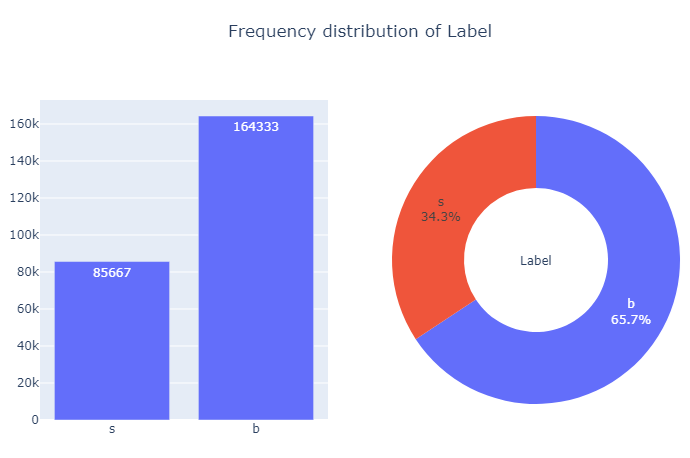
The target Label is a binary variable, taking values b and s, indicating the status of an event.
We present the frequency distribution of the target variable through barplot and donutplot.
Next, we check the number of unique values taken by the predictor variables in the following set of observations:
- Training observations that are background events
- Training observations that are signal events
- All training observations
- All test observations
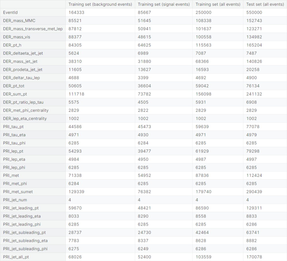
We observe that a lot of predictor variables take the value \(-999\) for a significant chunk of observations. The particular value is unnatural compared to the usual values taken by the variables. We suspect that the value is used for a crude imputation of missing or corrupted values.
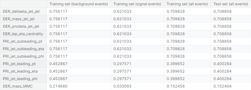
Now, we check the proportion of the value \(-999\) in the columns of the four sets of observations mentioned earlier.
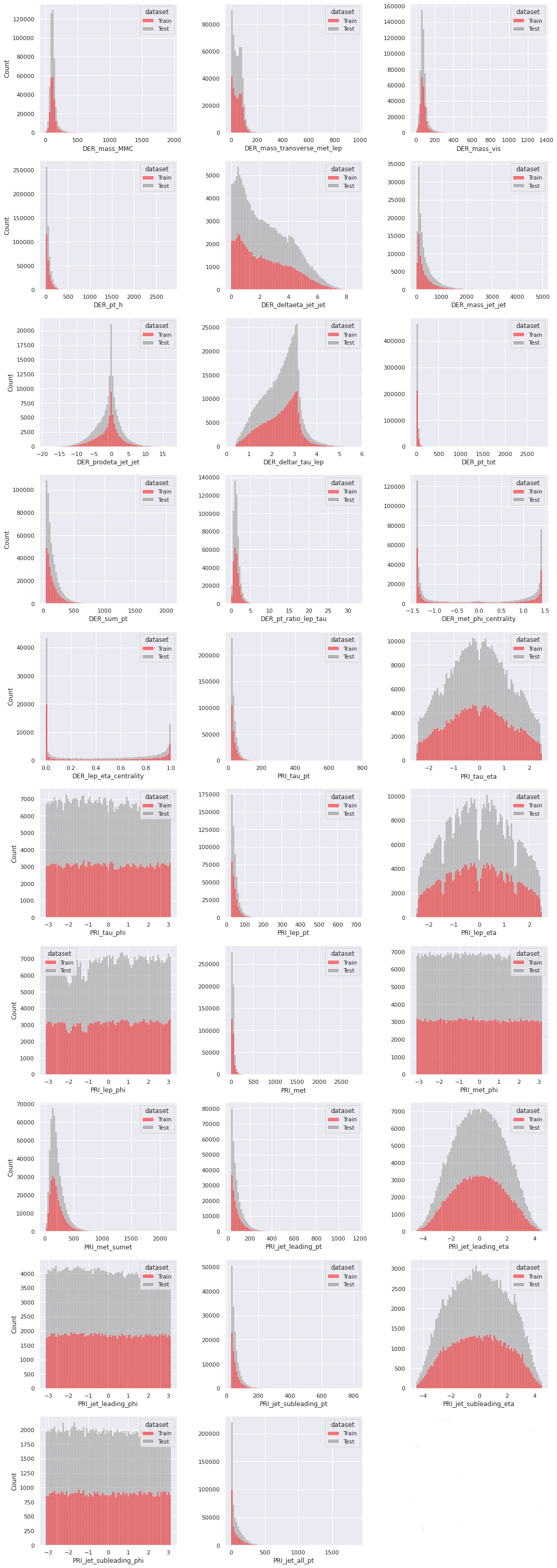
Next, we check the distributions of the float-type features for the training set and the test set. If we are to train our model on one set (the training set) and use it to make predictions on another (the test set), then it is desirable that the distributions corresponding to the two sets have similar structure. We replace the undesirable \(-999\)
values by np.nan, so that they do not distort the distributions.
Next, we compare the univariate distributions of the features for the background events and the signal events in the training set. If a feature has reasonably different distributions corresponding to the background events and the signal events, then it is a clear indication that the feature is important in the task of classifying the events when the label is unknown. Similarly, if a feature has very similar distributions for the two target classes, then it is unlikely to help in the classification problem based on the feature alone. This, however, does not take into account the possible dependence the feature may have with other features which may turn out to be useful in the task of classification. A multivariate analysis will be required to check that.
We present the distributions of the float features in the training set by the target class. As before, the \(-999\)
values are replaced by np.nan, so they do not affect the distributions.

Now, we check skewness of the distributions of the dataset columns. The measure quantifies the asymmetry of a distribution about its mean. It is given by
where \(\bar{x}\) is the mean of the observations, given by \(\bar{x} = \frac{1}{n}\sum_{i=1}^n x_i\).
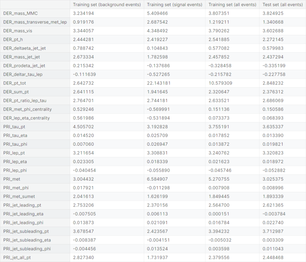
Observations
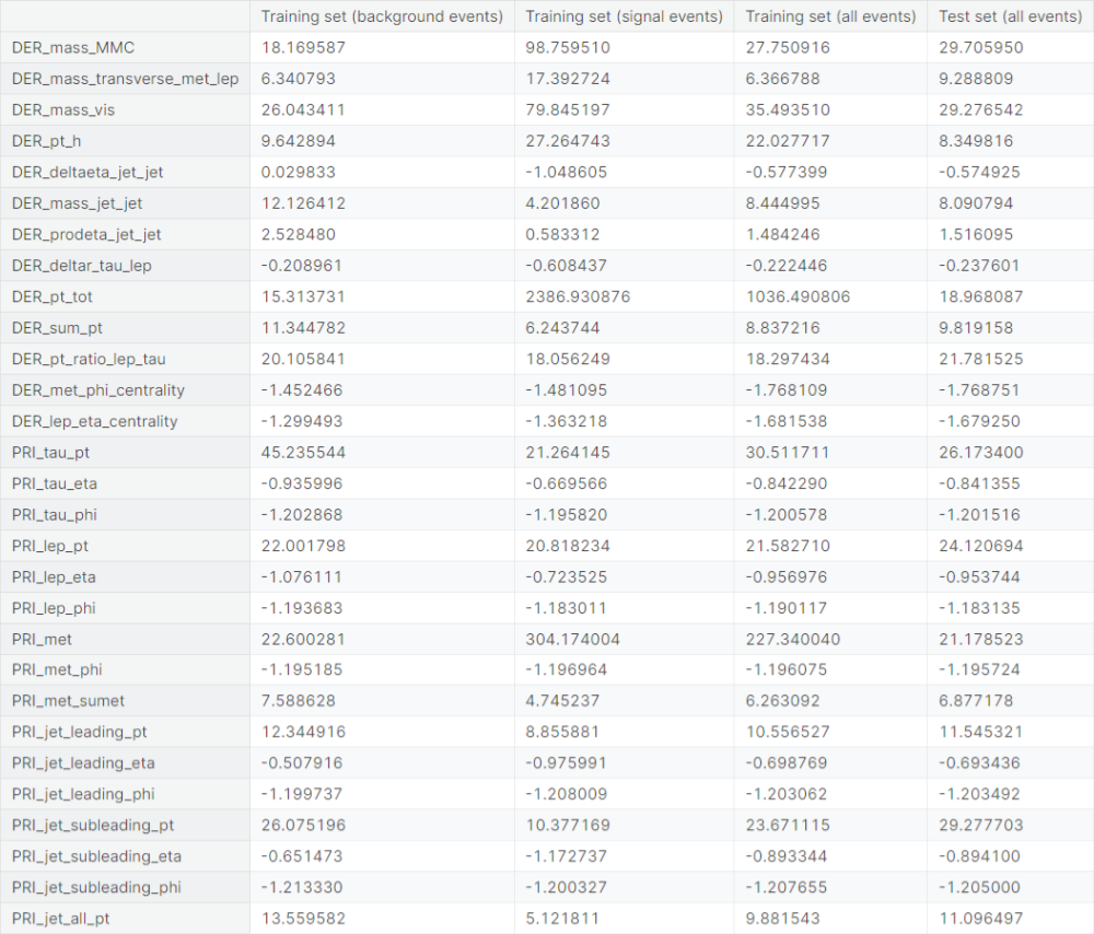
- Columns with extreme positive skewness (absolute value greater than \(3\)
in the training set):
DER_mass_MMC,DER_mass_vis,DER_pt_tot,PRI_tau_pt,PRI_lep_pt,PRI_met,PRI_jet_subleading_pt - Columns with high positive skewness (absolute value between \(1\)
and \(3\)
in the training set):
DER_mass_transverse_met_lep,DER_pt_h,DER_mass_jet_jet,DER_sum_pt,DER_pt_ratio_lep_tau,PRI_met_sumet,PRI_jet_leading_pt,PRI_jet_all_pt - Columns with moderate positive skewness (absolute value between \(0.5\)
and \(1\)
in the training set):
DER_deltaeta_jet_jet
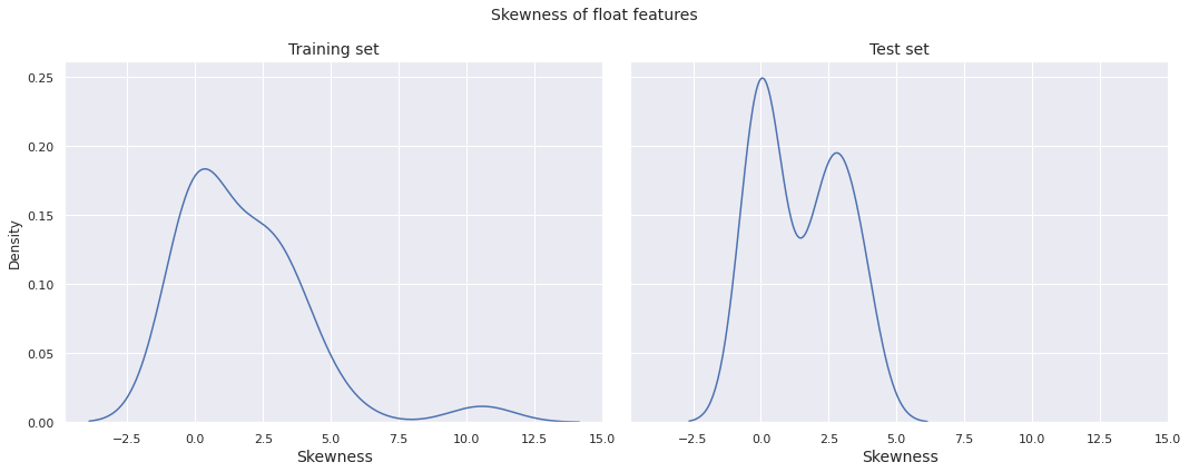
We plot the distribution of skewness of the float features in the training set and the test set.
Observations
- The skewness distribution for both the training set and the test set have global peak near \(0\)
- There is a mild peak far towards the right (around \(11\)) in the skewness distribution for the training set, indicating that some of the float features in the training set exhibit extremely high positive skewness
- The skewness distribution for the test set has a clear bimodal structure, with a local peak near \(2.5\)
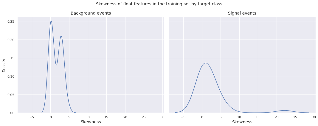
Next, we plot the distribution of skewness of the float features in the training set by target class.
Observations
- The skewness distribution for both the background events and the signal events in the training set have global peak near \(0\)
- There is a mild peak far towards the right (around \(22\)) in the skewness distribution for the signal events, indicating presence of float features with extreme positive skewness for the signal events
- The skewness distribution for the background events has a clear bimodal structure, with a local peak near \(2.5\)
Now, we check kurtosis of the distributions of the dataset columns. It generally quantifies the peakedness and tailedness of a distribution. It is given by
where \(\bar{x}\) is the mean of the observations, given by \(\bar{x} = \frac{1}{n}\sum_{i=1}^n x_i\). A relocated version of the kurtosis, taking into account the fact that \(b_2 = 3\) for the normal distribution is defined as the excess kurtosis, given by \(g_2 := b_2 - 3\).
Note: The ability of the measure \(b_2\) or \(g_2\) to quantify peakedness of a distribution has been a topic of debate. See this paper for more details.
Observations
- Columns with extreme leptokurtosis (excess kurtosis greater than \(3\)
in the training set):
DER_mass_MMC,DER_mass_transverse_met_lep,DER_mass_vis,DER_pt_h,DER_mass_jet_jet,DER_pt_tot,DER_sum_pt,DER_pt_ratio_lep_tau,PRI_tau_pt,PRI_lep_pt,PRI_met,PRI_met_sumet,PRI_jet_leading_pt,PRI_jet_subleading_pt,PRI_jet_all_pt - Columns with high leptokurtosis (excess kurtosis between \(1\)
and \(3\)
in the training set):
DER_prodeta_jet_jet - Columns with high platykurtosis (excess kurtosis between \(-3\)
and \(-1\)
in the training set):
DER_met_phi_centrality,DER_lep_eta_centrality,PRI_tau_phi,PRI_lep_phi,PRI_met_phi,PRI_jet_leading_phi,PRI_jet_subleading_phi - Columns with moderate platykurtosis (excess kurtosis between \(-1\)
and \(-0.5\)
in the training set):
DER_deltaeta_jet_jet,PRI_tau_eta,PRI_lep_eta,PRI_jet_leading_eta,PRI_jet_subleading_eta
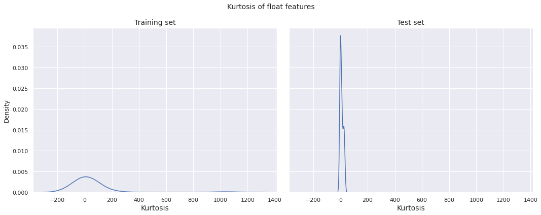
Now, we plot the distribution of kurtosis of the float features in the training set by target class.
Observations
- The kurtosis distribution for both the training set and the test set have global peak near \(0\)
- The kurtosis distribution for the training set is more or less bell-shaped and relatively dispersed, whereas the same for the test set is far more concentrated about \(0\) with high peakedness
Next, we plot the distribution of kurtosis of the float features in the training set by target class.
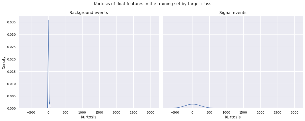
Observations
- The kurtosis distribution for both the background events and the signal events in the training set have global peak near \(0\)
- The kurtosis distribution for the signal events is more or less bell-shaped and relatively dispersed, whereas the same for the background events is far more concentrated about \(0\) with high peakedness
We also observe that for both skewness and kurtosis, there is an uncanny resemblance between the respective distribution plots for background events in the training set and all events in the test set. This indicates that majority of the observations in the test set may be background events.
We now turn our attention to the only integer feature PRI_jet_num. First, we present frequency comparison of PRI_jet_num for the training set and the test set.
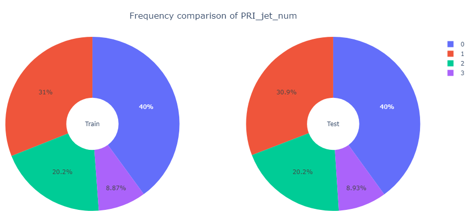
Observation: The proportions of values of PRI_jet_num are more or less same for both the training set and the test set.
Next, we present frequency comparison of PRI_jet_num for the background events and the signal events in the training set.
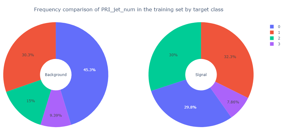
Observation: The proportions of values of PRI_jet_num, especially \(0\)
and \(2\),
differ for the background events and the signal events in the training set.
Multivariate Analysis
We begin with the correlation structure among the float features. Correlation coefficient is a statistical measure of linear dependence between two variables. Extreme correlation gives an indication that the two variables are linearly related, however this does not prove any causal relationship between the said variables. The measure is defined as the covariance of the two variables, scaled by the product of respective standard deviations. Let \(\left\{\left(x_1, y_1\right), \left(x_2, y_2\right), \cdots, \left(x_n, y_n\right)\right\}\) be paired data on the variables \(\left(x, y\right)\). Then the correlation coefficient of the two variables is given by
where \(\bar{x}\) and \(\bar{y}\) denote the respective sample means of the two variables, given by \(\bar{x} = \frac{1}{n}\sum_{i=1}^n x_i\) and \(\bar{y} = \frac{1}{n}\sum_{i=1}^n y_i\).

We plot the distributions of correlation coefficient of pairs of float features for the training set and the test set.
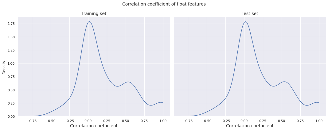
Observations
- The correlation distribution is almost identical for the training set and the test set
- The density has its global peak near \(0\), however there is a local peak between \(0.5\) and \(0.6\), indicating a fair number of moderately to highly correlated pairs of features
- There is even an increase in the density after \(0.8\), with a small peak very close to \(1\), indicating the presence of a few extremely correlated pairs of features
We present the correlation heatmap of the float features in the training set.
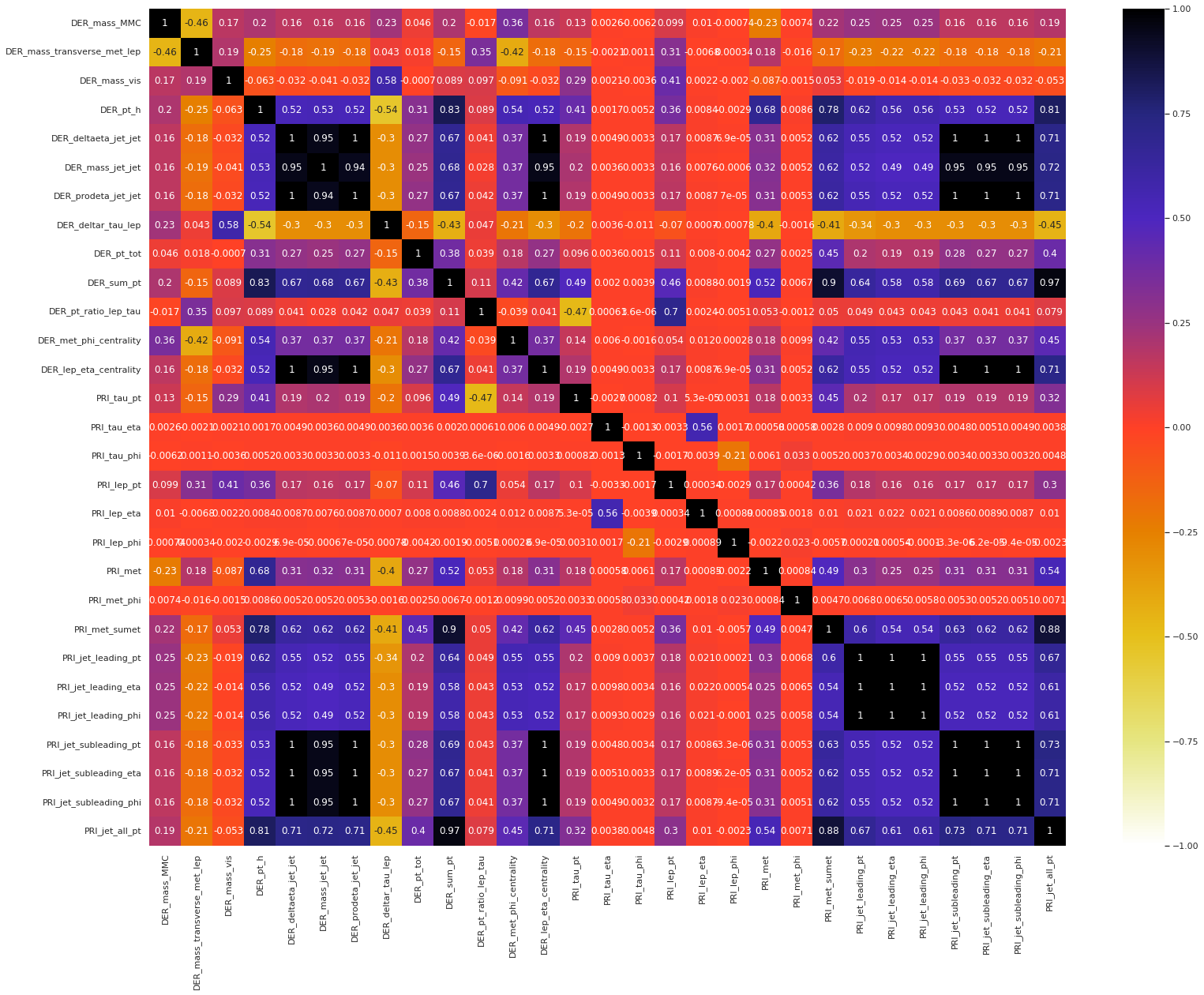
Next, we present the correlation heatmap of the float features in the test set.

Observation: The following groups have shown an extremely high positive correlation structure within themselves, i.e., any two features from a single group have an extremely high correlation coefficient.
DER_deltaeta_jet_jet,DER_mass_jet_jet,DER_prodeta_jet_jet,DER_lep_eta_centrality,PRI_jet_subleading_pt,PRI_jet_subleading_eta,PRI_jet_subleading_phiDER_sum_pt,PRI_met_sumet,PRI_jet_all_ptPRI_jet_leading_pt,PRI_jet_leading_eta,PRI_jet_leading_phi
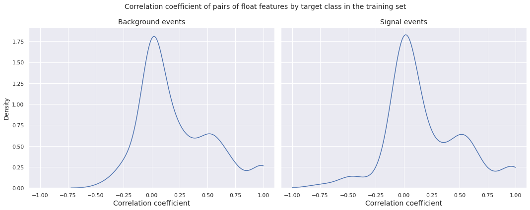
Now, we plot the distributions of correlation coefficient of pairs of float features by target class in the training set.
Observations
- The left tail of the correlation distributions corresponding to background events and signal events in the training set are different
- The densities have their respective global peaks near \(0\), however there is a local peak between \(0.5\) and \(0.6\) for both of them, indicating a fair number of pairs of float features with moderate to high positive correlation
- The left tail of the correlation distribution for the signal events is heavier compared to the same for the background events, indicating that there are more pairs of float features with moderate to high negative correlation for the signal events than the background events in the training set
- For both target classes, there is an increase in the density after \(0.8\), with a small peak very close to \(1\), indicating the presence of a few pairs of float features with extreme positive correlation
We present the correlation heatmaps of the float features for background events and signal events in the training set.
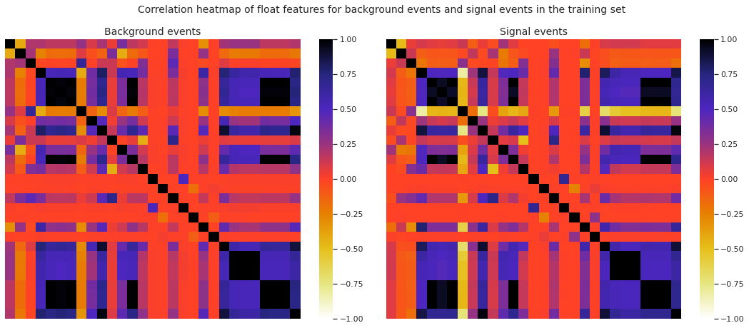
Observation: The two heatmaps are more or less similar, i.e., the overall correlation structure of the float features corresponding to the background events and the signal events in the training set are very much alike.
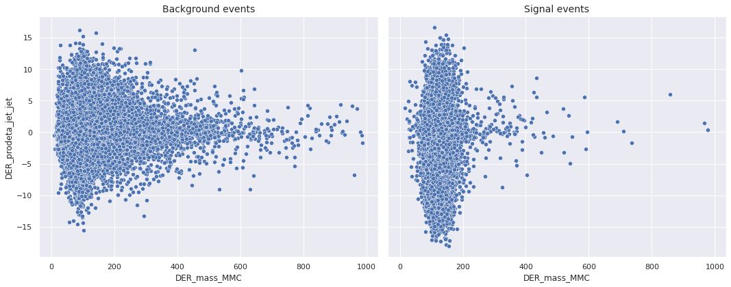
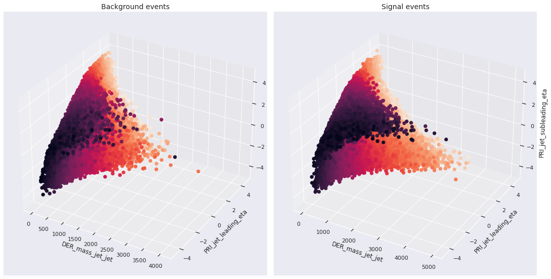
In this notebook, we present bivariate (trivariate) scatterplots for some selected pairs (triples) of features. These plots are given separately for the background events and signal events appearing in the training set. So they can be used not only to understand the relationship between (among) a pair (triple) of features, but also the ability of the pair (triple) to classify an event as background or signal.
For the sake of brevity, we do not show all the plots in this post. Instead, we give one example of bivariate scatterplot and one example of trivariate scatterplot. First, we present the bivariate scatterplot of DER_mass_MMC and DER_prodeta_jet_jet.
Now, we present the trivariate scatterplot of DER_mass_jet_jet, PRI_jet_leading_eta, and PRI_jet_subleading_eta.
○ Train-Test Split
The original test set does not contain Weight and Label. It is useful only in the context of this competition. Thus, we cannot utilize it to evaluate the models in this project. Instead, we take a chunk out of the training set and hold it out for final evaluation.
Specifically, we split the original training set in \(80:20\) ratio. The new training set consists of \(80\%\) training data, and the new test set consists of the rest.
We stratify the split using Label, so that the proportion of each label remains roughly the same in the new training set and the new test set.
○ Data Preprocessing
Categorical Data Encoding
We observe that the labels are nominal in nature, i.e., they do not have an inherent order. To encode the labels, we map them to integer values in the following way: \(\text{b} \mapsto 0\) and \(\text{s} \mapsto 1\).
The values of the Label column in both the training set and the test set are replaced with the corresponding encoded values.
Dropping Redundant Columns
The EventId column has no relevance as far as the classification problem under consideration is concerned. So, we drop it from both the training set and the test set.
We have observed in the exploratory data analysis that \(11\) columns in the dataset contain the value \(-999\), which is very different from the other values taken by the respective features. We suspect that these are missing values filled in by a constant of arbitrary choice.
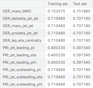
We drop these columns from the dataset. One can also experiment by imputing the \(-999\)
values in the column DER_mass_MMC, which has a little over \(15\%\)
values equal to \(-999\).
Furthermore, we have observed in the exploratory data analysis that the following groups have shown extremely high positive correlation structure within themselves, i.e., any two features from a single group has extremely high correlation coefficient.
DER_deltaeta_jet_jet,DER_mass_jet_jet,DER_prodeta_jet_jet,DER_lep_eta_centrality,PRI_jet_subleading_pt,PRI_jet_subleading_eta,PRI_jet_subleading_phiDER_sum_pt,PRI_met_sumet,PRI_jet_all_ptPRI_jet_leading_pt,PRI_jet_leading_eta,PRI_jet_leading_phi
The first group and the last group are subsets of the dropped columns. We can explain the extremely high correlation between the pairs in those groups by the high frequency of the value \(-999\).
The middle group of three features, though, does not have the same explanation. We keep only DER_sum_pt from these columns and drop the other two.
○ Feature Engineering
Transformation
We note the following observations from the exploratory data analysis.
- Columns with extreme skewness (absolute value greater than \(3\)
in the dataset):
DER_mass_MMC,DER_mass_vis,DER_pt_tot,PRI_tau_pt,PRI_lep_pt,PRI_met,PRI_jet_subleading_pt - Columns with high skewness (absolute value between \(1\)
and \(3\)
in the dataset):
DER_mass_transverse_met_lep,DER_pt_h,DER_mass_jet_jet,DER_sum_pt,DER_pt_ratio_lep_tau,PRI_met_sumet,PRI_jet_leading_pt,PRI_jet_all_pt - Columns with moderate skewness (absolute value between \(0.5\)
and \(1\)
in the dataset):
DER_deltaeta_jet_jet
In this project, we shall transform all the features with absolute value of skewness more than \(0.5\).
It turns out that these columns are DER_mass_transverse_met_lep, DER_mass_vis, DER_pt_h, DER_pt_tot, DER_sum_pt, DER_pt_ratio_lep_tau, PRI_tau_pt, PRI_lep_pt, and PRI_met.
The next function transforms the selected input columns of two input DataFrames in the following manner:
- First, it applies location change \(x \mapsto x - min(x) + 1\) on the features to be transformed, to make their range start from \(1\). The relocated variables fall inside the range \([1, \infty)\).
- Now we apply the log transformation \(y \mapsto \log{y}\).
def log_transform(df_train_in, df_test_in, cols_transform):
    df_train_out, df_test_out = df_train_in.copy(deep = True), df_test_in.copy(deep = True)
    for col in cols_transform:
        min_ = df_train_out[col].min()
        df_train_out[col] = df_train_out[col] - min_ + 1
        df_train_out[col] = np.log(df_train_out[col])
        df_test_out[col] = df_test_out[col] - min_ + 1
        df_test_out[col] = np.log(df_test_out[col])
    return df_train_out, df_test_out
The relocation preceding the log transformation ensures that there are no negative values to be fed to the \(\log\) function. The addition of \(1\) ensures that there are no values very close to \(0\), which the log transformation maps to extreme negative values.
Note that we use the same \(\min(x)\) from the training data in the test data, to keep the transformation same for the two datasets.
Feature Scaling
It may be natural for one feature variable to have a greater impact on classification procedure than another. But often this is generated artificially by the difference of range of values that the features take. The unit of measurement in which the features are measured can be one a possible reason for such occurrence.
To deal with this, the min-max normalization transforms the features in the following way:
The following function applies min-max normalization on selected columns of an input training DataFrame and an input test DataFrame. To keep the transformation the same, we use the minimum and maximum values of the training columns only for both DataFrames. Using the minimum and maximum values of the test columns for both sets would have led to data leakage.
Specifically, we compute \(\min{\left(x\right)}\) and \(\max{\left(x\right)}\) for a particular feature from the training set only, and use those values to rescale the feature for both the training set and the test set.
def minmax_normalizer(df_train_in, df_test_in, cols):
    df_train_out, df_test_out = df_train_in.copy(deep = True), df_test_in.copy(deep = True)
    for col in cols:
        min_, max_ = df_train_out[col].min(), df_test_out[col].max()
        df_train_out[col] = (df_train_out[col] - min_) / (max_ - min_)
        df_test_out[col] = (df_test_out[col] - min_) / (max_ - min_)
    return df_train_out, df_test_out
We employ normalization on the non-constant float features in the training set and the test set.
○ Baseline Model
- Model Creation and Compilation
- Early Stopping
- Learning Rate Scheduler
- Model Checkpoint
- Model Fitting
- Label Prediction
- Model Evaluation
First, we split both the training set and the test set into features, label, and weight.
Model Creation and Compilation
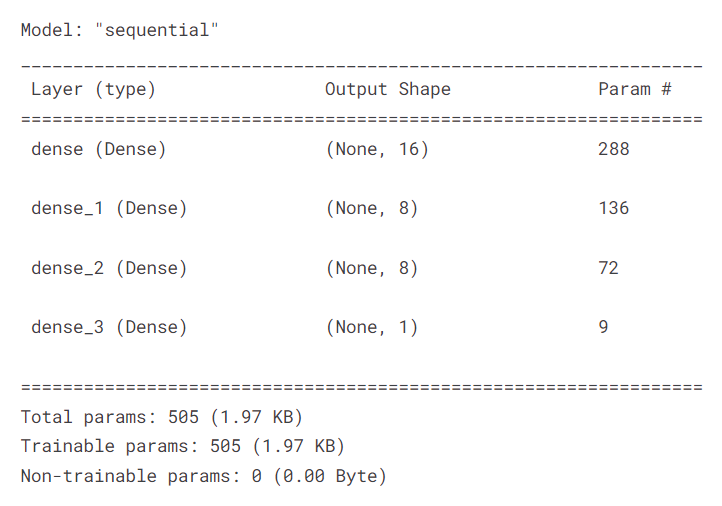
The next function creates a model and compiles it. Specifically, it adds dense layers, with appropriate number of units and activation function, to a sequential model. Then, it compiles the model with binary cross-entropy loss and Adam optimizer with an input learning rate. The model is evaluated with the accuracy metric during the training process.
def createModel(learning_rate = 0.001):
    model = Sequential()
    model.add(Dense(units = 16, input_dim = len(X_train.columns), activation = 'relu'))
    model.add(Dense(units = 8, activation = 'relu'))
    model.add(Dense(units = 8, activation = 'relu'))
    model.add(Dense(units = 1, activation = 'sigmoid'))
    model.compile(loss = 'binary_crossentropy',
                  optimizer = tf.keras.optimizers.Adam(learning_rate = learning_rate),
                  metrics = ['accuracy'])
    return model
We apply the function and report the summary of the model.
model = createModel()
model.summary()
Early Stopping
The early stopping callback is useful in stopping the training process once it reaches a certain level of stagnation.
We create an instance of the callback, which monitors the validation loss and stops the training process if the validation loss does not change beyond the amount \(0.001\) for \(20\) epochs.
earlystop = EarlyStopping(
    monitor = 'val_loss',
    min_delta = 0.001,
    patience = 20,
    verbose = 0,
    mode = 'auto',
    start_from_epoch = 60
)
Learning Rate Scheduler
A learning rate scheduler modifies the learning rate during the training process, frequently decreasing it as the training goes on. This allows better fine-tuning by enabling the model to make larger updates early in the training process when the parameters are far from optimal and smaller updates later on when the parameters are closer to optimal.
At the beginning of every epoch, this callback gets the updated learning rate value from a schedule function, with the current epoch and current learning rate, and applies the updated learning rate on the optimizer. The schedule function takes an epoch index (integer, indexed from 0) and current learning rate (float) as inputs and returns a new learning rate as output (float).
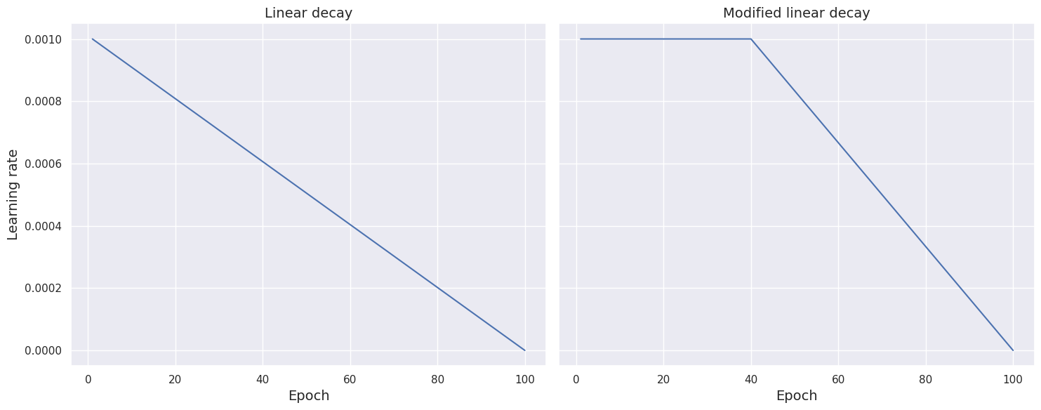
Modified linear schedule function. A common choice of scheduler is linear decay. In what follows, we manually set the total number of epochs to \(100\).
This can be modified as per requirement. Thus, unless interrupted by the early stopping callback, the training process runs from epoch = 0 to epoch = 99. The following function implements the linear decay, where the learning rate linearly decreases as the training process approaches the \(100\)th
epoch.
def scheduler_linear(epoch, learning_rate):
    if epoch < 1:
        return learning_rate
    else:
        return learning_rate * (100 - epoch - 1) / (100 - epoch)
The next function modifies the scheduler by keeping the learning rate constant for the first \(40\) epochs and then gradually decreasing it at a linear rate as it approaches the \(100\)th epoch. Note that we manually set the initial number of epochs (when the learning rate remains the same) to \(40\). This can be changed as per need.
def scheduler_modified_linear(epoch, learning_rate):
    if epoch < 40:
        return learning_rate
    else:
        return learning_rate * (100 - epoch) / (100 - epoch + 1)
We compare the two schedule function by plotting learning rate against epoch for both setup.
Modified exponential schedule function. Another common choice of scheduler is exponential decay. The following function implements the scheduler, which decreases the learning rate exponentially as the training process approaches the \(100\)th epoch.
def scheduler_exponential(epoch, learning_rate):
    if epoch < 1:
        return learning_rate
    else:
        return learning_rate * math.exp(-0.1)
The next function modifies the scheduler by keeping the learning rate constant for the first \(40\) epochs and then gradually decreasing it at an exponential rate as it approaches the \(100\)th epoch.
def scheduler_modified_linear(epoch, learning_rate):
    if epoch < 40:
        return learning_rate
    else:
        return learning_rate * (100 - epoch) / (100 - epoch + 1)
We compare the two schedule function by plotting learning rate against epoch for both setup.
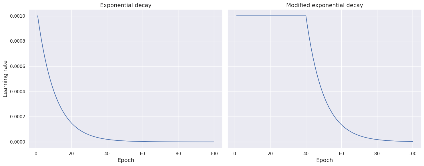
In this project, we use the modified linear decay.
learning_rate_scheduler = LearningRateScheduler(scheduler_modified_linear)
Model Checkpoint
The ModelCheckpoint callback saves a Keras model or model weights at some frequency. It works together with training using model.fit() to save a model or weights (in a checkpoint file) at certain interval. This allows the model or weights to be loaded at a later time to resume training from the saved state.
Here, we only keep the model that has achieved the best performance so far, in terms of validation loss, instead of saving the model at the end of every epoch regardless of performance.
model_checkpoint = ModelCheckpoint(
    filepath = 'best_model.h5',
    monitor = 'val_loss',
    save_best_only = True
)
Model Fitting
We incorporate the three callbacks described above in training the model for \(100\) epochs, taking \(32\) observations per gradient update.
Specifically, we set aside the last \(20\%\) observations from the training set to constitute the validation set. The rest constitutes the effective training set. In each epoch, the model is trained over the effective training set and is evaluated on the validation set.
history = model.fit(
    X_train,
    y = y_train,
    batch_size = 32,
    epochs = 100,
    validation_split = 0.2,
    callbacks = [earlystop, learning_rate_scheduler, model_checkpoint],
    verbose = 0
)
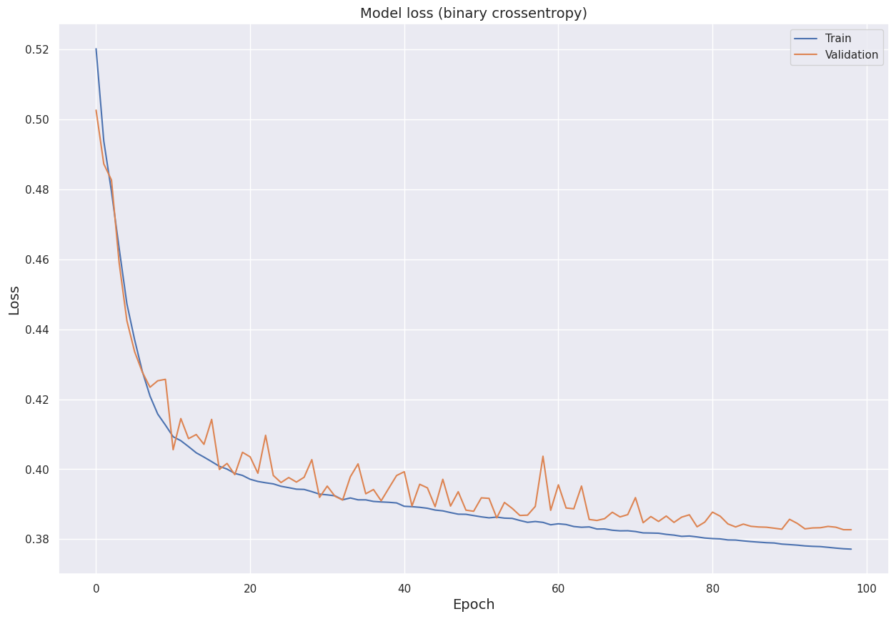
We visualize the model loss (binary cross-entropy) for the training set and the validation set over the epochs.
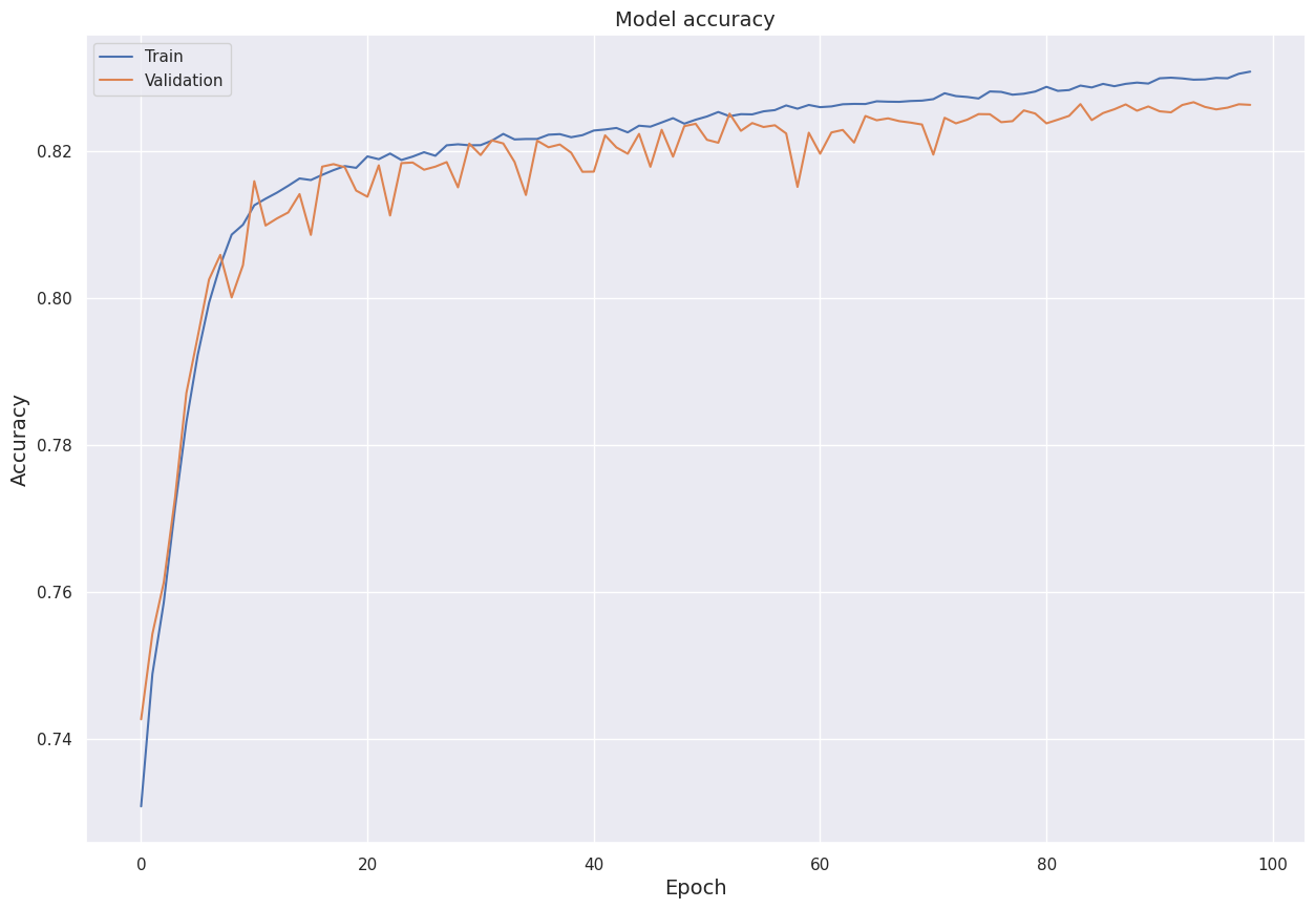
Furthermore, we visualize model accuracy for the training set and the validation set over the epochs.
Label Prediction
We load the best model, which is saved by the ModelCheckpoint callback, to predict the label \(1\)
(signal event) probabilities. Then, we convert them to binary predictions (\(0\)
or \(1\)).
Model Evaluation
We compute approximate median significance (AMS) for predictions on the training set and the test set.
- Training AMS: \(2.509776\)
- Test AMS: \(1.214260\)
○ Hyperparameter Tuning
Keras Model
We employ the scikit-learn classifier API for Keras, KerasClassifier, to create and compile the model.
The createModel function, defined earlier, is used to build the Keras model, compiled using the Adam optimizer and binary cross-entropy loss. The model is set to train for \(100\)
epochs, taking \(32\)
observations per gradient update. As before, we incorporate the three callbacks: EarlyStopping, LearningRateScheduler, and ModelCheckpoint. We fix the random_state parameter for reproducibility of the results.
model_ = KerasClassifier(
    model = createModel,
    optimizer = 'adam',
    loss = 'binary_crossentropy',
    batch_size = 32,
    epochs = 100,
    learning_rate = 0.001,
    callbacks = [earlystop, learning_rate_scheduler, model_checkpoint],
    random_state = 0,
    verbose = 0
)
Grid Search
We employ the traditional grid search technique for hyperparameter tuning. We shall focus on tuning two specific parameters, namely batch_size and learning_rate. The following dictionary contains the specific values of these parameters during the grid search.
param_grid = {
    'batch_size'   : [32, 64, 128],
    'learning_rate': [0.001, 0.003, 0.01]
}
We feed this to the GridSearchCV class, which trains the model from each of the \(3 \times 3 = 9\)
instances in param_grid. The \(5\)-fold
cross-validated models are evaluated by the accuracy metric and the best model is refit to the entire training set.
Best Model Instance
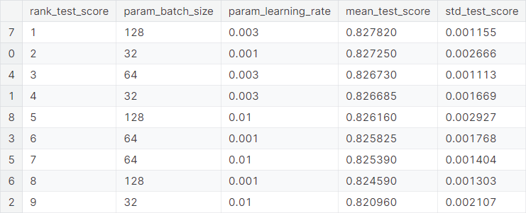
The optimal values of the hyperparameters are given as follows.
batch_size: \(128\)learning_rate: \(0.003\)
The best cross-validation score, which is \(5\)-fold cross-validation accuracy in this case, is \(0.82782\).
○ Prediction and Evaluation
We predict the label \(1\) (signal event) probabilities using the tuned model and convert the predicted probabilities to labels. The AMS scores for predictions on the training set and the test set are computed.
- Training AMS: \(2.500144\)
- Test AMS: \(1.200022\)
Observe that the test AMS for the tuned model is actually less than that of the baseline model, which may prompt one to suspect that it is a poorer model. However, it is not the case, as the candidates for the tuned model were evaluated under a cross-validation setup where the final model has the highest cross-validation score, exceeding that of the baseline model.
While the performance (in terms of AMS score) does dip very slightly on the particular test set, we aim to produce a model that generalizes best to new data. For that reason, we go with the model that gives the best cross-validation score.
Next, we compute accuracy scores for predictions on the training set and the test set. Note that accuracy does not consider Weight of the observations.
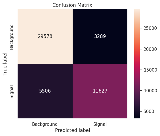
- Training accuracy: \(0.827070\)
- Test accuracy: \(0.824100\)
Finally, we produce a confusion matrix that depicts the performance of the final model on the test set.
○ Acknowledgements
- Dataset from the ATLAS Higgs Boson Machine Learning Challenge \(2014\)
- Higgs Boson Machine Learning Challenge dataset
- The Higgs boson machine learning challenge documentation
○ References
- Activation function
- Adam optimizer
- ATLAS
- Binary cross-entropy
- Boson
- CERN
- Confusion matrix
- Correlation coefficient
- Data leakage
- Deep learning
- Deep neural networks
- Dense layers
- Early stopping
- Elementary particle
- Evaluation of binary classifiers
- Evidence for Higgs Boson Decays to the \(\tau^+\tau^-\) Final State with the ATLAS Detector
- Excess kurtosis
- Exploratory data analysis
- False positive rate
- Fermion
- Fundamental interaction
- Grid search
- Higgs boson
- Hyperparameter optimization
- Indicator function
- Keras
- Kurtosis
- Kurtosis as Peakedness, \(1905–2014\). R.I.P.
- Learning rate
- Learning rate scheduler
- Logarithm
- Machine learning
- Min-max normalization
- Missing data
- Model checkpoint
- Natural logarithm
- Neural network
- Nominal category
- Normal distribution
- Order theory
- Particle accelerator
- Particle beam
- Particle decay
- Particle physics
- Scikit-learn
- Sensitivity and specificity
- Sequential model
- Skewness
- Stratified sampling
- Subatomic particle
- Tau lepton
- The HiggsML challenge
- Test dataset
- Training dataset
- Train-test split