Electron Energy Flux Prediction
In McGranaghan et al. (2021), the authors considered the problem of modeling electron particle precipitation from the magnetosphere to the ionosphere. They attempted to address the problem through a new particle precipitation database, using machine learning tools to extract useful information from it. The new database contains 51 satellite years of Defense Meteorological Satellite Program (DMSP) observations. Based on this, we aim to predict the continuous target variable electron total energy flux.
○ Contents
- Overview
- Introduction
- Exploratory Data Analysis
- Data Preprocessing
- Baseline Neural Network
- Hyperparameter Tuning
- Prediction and Evaluation
- Acknowledgements
- References
○ Overview
- In McGranaghan et al. (2021), the authors have considered the problem of modeling electron particle precipitation from the magnetosphere to the ionosphere. They attempted to address it through a new database, using machine learning tools to extract useful information from it.
- Based on that database, we aim to predict electron total energy flux, which is a continuous variable.
- A detailed exploratory data analysis on the dataset is carried out. In particular, we observe that there are clear groups among the feature variables. We investigate the group-wise correlation structure through averaging the pairwise correlation coefficients.
- We use the insights obtained from EDA in the data preprocessing stages, which consists of feature extraction, data transformation, feature scaling, and principal component analysis.
- We build a neural network and tune it to predict electron total energy flux.
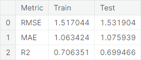
- We employ the root mean square error (RMSE), mean absolute error (MAE), and coefficient of determination (\(R^2\)) metrics to evaluate the models. Performance summary of the final model:
○ Introduction
Data
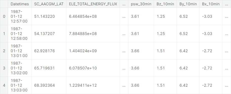
The dataset accompanies this paper published in the AGU Space Weather Journal and is used to produce new machine learning models of particle precipitation from the magnetosphere to the ionosphere. The authors have attempted to make these data ready to be used in artificial intelligence or machine learning explorations, following a community definition of AI-ready provided at this repository. The dataset contains \(1945789\) observations, each containing \(74\) variables.
Project Objective
The goal is to predict ELE_TOTAL_ENERGY_FLUX, which is a continuous variable, based on the features available in the dataset.
Evaluation Metric
We use the trained models to predict on the test dataset and evaluate the models in terms of root mean square error (RMSE), mean absolute error (MAE), and coefficient of determination (\(R^2\)).
○ Exploratory Data Analysis
Dataset Synopsis
- Number of observations: \(1945789\)
- Number of columns: \(74\)
- Number of integer columns: \(0\)
- Number of float columns: \(73\)
- Number of object columns: \(1\)
- Number of duplicate observations: \(0\)
- Constant columns: None
- Number of columns with missing values: \(0\)
- Memory Usage: \(1098.54\) MB
Univariate Analysis
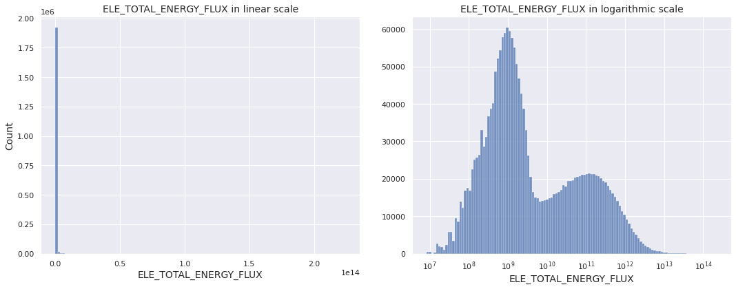
We visualize the distribution of the continuous target variable ELE_TOTAL_ENERGY_FLUX through histogram and observe that it is extremely skewed in linear scale. So, we set log_scale = True in seaborn histplot and visualize the distribution on logarithmic scale.
Observations
- The target variable has extremely left-skewed distribution, which suggests applying log-transformation \(y \mapsto \log{y}\) on it
- Under logarithmic scale, the distribution appears to be bimodal
Next, we visualize the distributions of the numerical features.

Observations
- Extremely skewed columns:
ELE_AVG_ENERGY - Moderately skewed columns:
ELE_TOTAL_ENERGY_FLUX_STD,ELE_AVG_ENERGY_STD,F107,AE,AU,F107_6hr,AE_6hr,AU_6hr,psw_6hr,F107_5hr,AE_5hr,AU_5hr,PC_5hr,psw_5hr,F107_3hr,AE_3hr,AU_3hr,psw_3hr,F107_1hr,AE_1hr,AU_1hr,psw_1hr,F107_45min,AE_45min,AU_45min,psw_45min,F107_30min,AE_30min,AU_30min,psw_30min,F107_15min,AE_15min,AU_15min,psw_15min,F107_10min,AE_10min,AU_10min,psw_10min,F107_5min,AE_5min,AU_5min,psw_5min - Extremely leptokurtic columns:
PC_6hr,PC_5hr,PC_3hr,PC_1hr - Moderately skewed columns taking negative values:
AL,psw,AL_6hr,AL_5hr,AL_3hr,AL_1hr,AL_45min,AL_30min,AL_15min,AL_10min,AL_5min - Columns with zero-inflated distribution:
borovsky,newell,borovsky_45min,newell_45min,borovsky_30min,newell_30min,borovsky_15min,newell_15min,borovsky_10min,newell_10min,borovsky_5min,newell_5min
Multivariate Analysis
Barring the object type variable Datetimes, all the features are of the float datatype. We begin with investigating the pairwise correlation coefficients for the numerical feature variables.
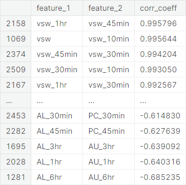
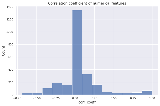
We present a histogram of the pairwise correlation coefficient values to give an overall picture of the extention of the correlation among the numerical features in the dataset.
Observations
- In total there are \(\binom{152}{2} = 11476\) pairs of numerical features
- No significant correlation \((\left\vert r \right\vert < 0.1):\) \(6061\) pairs
- Weak correlation \((0.1 \leq \left\vert r \right\vert < 0.3):\) \(3195\) pairs
- Moderate correlation \((0.3 \leq \left\vert r \right\vert < 0.7):\) \(1653\) pairs
- Strong correlation \((0.7 \leq \left\vert r \right\vert < 0.9):\) \(222\) pairs
- Extremely strong correlation \((0.9 \leq \left\vert r \right\vert < 0.99):\) \(238\) pairs
- Almost linear relationship \((0.99 \leq \left\vert r \right\vert \leq 1):\) \(107\) pairs
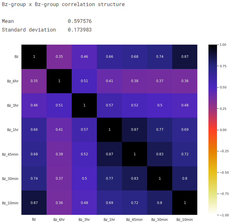
We observe that there are clear groups among the feature variables, as indicated by their names starting with certain common strings. For example, the features Bz, Bz_6hr, Bz_3hr, Bz_1hr, Bz_45min, Bz_30min, and Bz_10min appears to be related in some sense. We consider these different groups of features and investigate the group-wise correlation structure through averaging the pairwise correlation coefficients.
To elaborate, let us take a group \(G_1\) of the features \(X_1, X_2, \cdots, X_m\). We can now define the mean of within-group correlation coefficient as
We define the variance of within-group correlation coefficient as
Now, let us take another group \(G_2\) of the features \(Y_1, Y_2, \cdots, Y_n\). Note that the group sizes of \(G_1\) and \(G_2\) do not necessarily have to be equal. We define the mean of between-group correlation coefficient as
We define the variance of between-group correlation coefficient as
These measures prove to be useful in the group-wise analysis of the correlation structure among numerical features. We begin with forming different groups of features.
group_list = [col.split("_")[0] for col in data.columns if '_6hr' in col]
group_dict = {}
for item in group_list:
    group_dict[item] = [col for col in data.columns if item in col]
group_dict['AL'].remove('ELE_TOTAL_ENERGY_FLUX')
We illustrate the correlation structure among the groups through average pairwise correlation coefficients with a heatmap.
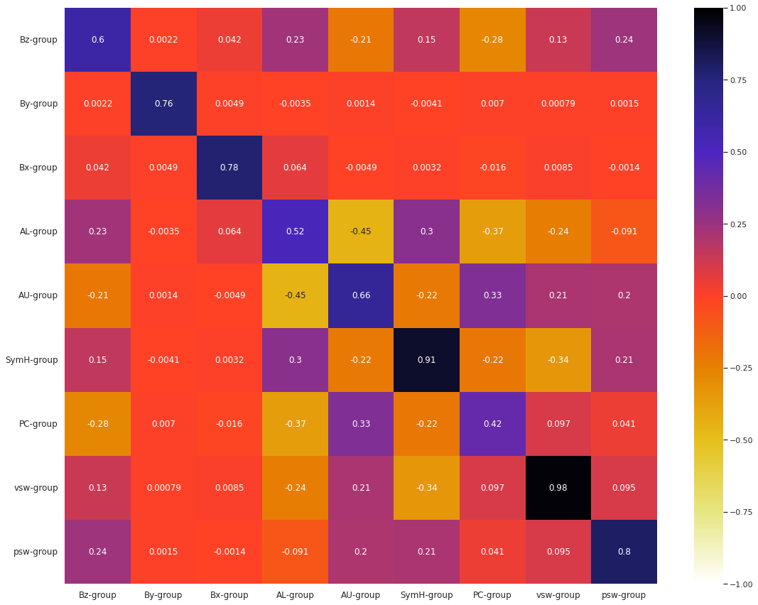
Note that the diagonal elements of the group-wise correlation matrix is not necessarily equal to \(1\), unlike the case of usual correlation matrices. This is because, in this scenario, the diagonal elements represent the average pairwise correlation coefficient of a group of features, instead of the correlation coefficient of a feature with itself.
To illustrate how this grouped heatmap works, we give an in-depth view of the top-left square, which shows the average correlation coefficient within the Bz-group.
Observations from the grouped heatmap
-
The diagonal squares show that all the groups have moderate to high average correlation among its features (taken as pairs). We shall take in-depth look into each of the groups.
-
The non-diagonal squares show that the average correlation between different groups varies from extremely negative to moderately positive. Some squares with strong (positive or negative) correlation, which we may want to look into, are given in
first group\(\times\)second groupformat:vsw-group\(\times\)vx-groupAE-group\(\times\)AL-groupAE-group\(\times\)AU-groupAL-group\(\times\)AU-groupAE-group\(\times\)newell-groupAE-group\(\times\)PC-groupBz-group\(\times\)newell-groupAU-group\(\times\)newell-groupAL-group\(\times\)PC-groupAL-group\(\times\)newell-groupSymH-group\(\times\)vsw-groupSymH-group\(\times\)vx-groupPC-group\(\times\)newell-groupAU-group\(\times\)PC-groupborovsky-group\(\times\)newell-groupBz-group\(\times\)borovsky-groupAL-group\(\times\)SymH-group
The detailed visualizations for correlation structure within groups and between groups are available in this notebook.
○ Data Preprocessing
- Feature Extraction from
Datetimes - Log-transformation of the Target
- Feature Scaling
- Principle Component Analysis (PCA)
The preprocessing of data is carried out in four stages. We postpone the train-test split until the end of the second stage, as the first two stages have no scope of data leakage.
Feature Extraction from Datetimes
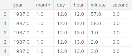
A typical value of the object type feature variable Datetimes looks like 1987-01-12 12:57:00. Clearly, it contains information on
- Year
- Month
- Day
- Hour
- Minute
- Second
We separate out these information as new features and subsequently drop the original Datetimes column from the dataset. A snapshot of the new features is given as follows:
Next, we give statistical description of the new features.

We drop the constant column second from the dataset.
Log-transformation of the Target
We observed in the exploratory data analysis that the target variable ELE_TOTAL_ENERGY_FLUX has an extremely left-skewed distribution. Thus, we transform the target by applying the map \(y \mapsto \log{y}\).
Train-Test Split. We split the dataset into training set and test set in \(80 : 20\) ratio. The training set contains \(1556631\) observations and the test set contains \(389158\) observations, each having \(77\) variables.
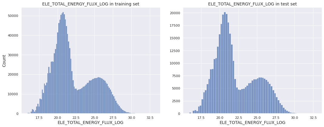
The distributions of the log-transformed target variable in the training set and test set are shown in the next diagram. The two distributions appear to be similar.
Feature Scaling
It may be natural for one feature variable to have a greater impact on classification procedure than another. But often this is generated artificially by the difference of range of values that the features take. The unit of measurement in which the features are measured can be one a possible reason for such occurrence.
This necessitates the practitioner to scale the features appropriately before feeding the data to machine learning algorithms. For this purpose, the min-max normalization transforms the features in the following way:
The next function implements this using the MinMaxScaler class from the scikit-learn library. To keep the transformation the same, we use the minimum and maximum values of the training columns to scale the corresponding columns in both the training set and the test set. Using the minimum and maximum values of the test columns for both datasets would have led to data leakage.
def scaler(X_train, X_test):
    scaling = MinMaxScaler().fit(X_train)
    X_train_scaled = scaling.transform(X_train)
    X_test_scaled = scaling.transform(X_test)
    return X_train_scaled, X_test_scaled
Principle Component Analysis (PCA)
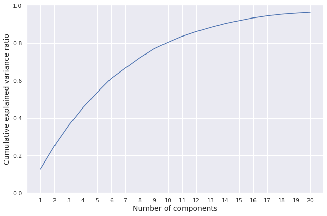
We import the PCA class from the scikit-learn library and fit it on the training features. We set the argument n_components (the number of components to keep) to \(20\).
The number of components kept and the ratio of variance explained by the retained components are summarized below.

We plot the cumulative explained variance ratio over the number of components.
A snapshot of the correlation structure of components and features is given as follows.

Next, we PCA-transform the training set features and give a snapshot of the transformed data.

Similarly, we PCA-transform the test set features and give a snapshot of the transformed data.

○ Baseline Neural Network
Model Creation
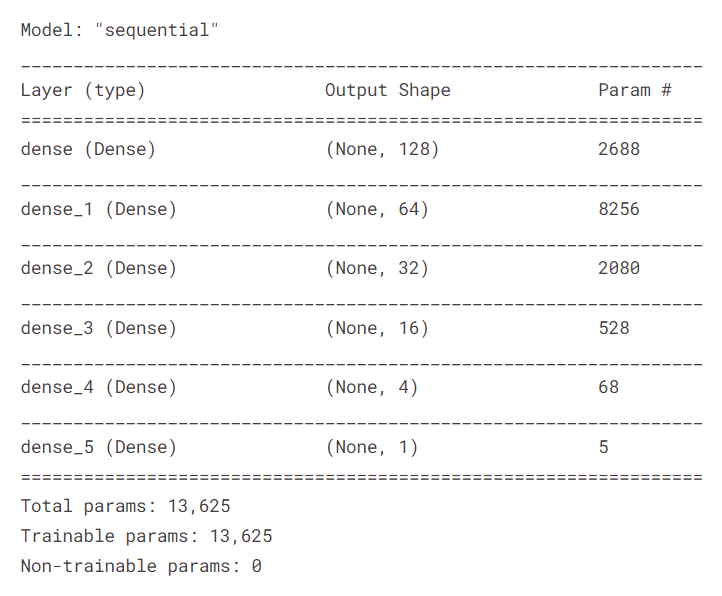
We add dense layers, with appropriate number of units and activation function, to a sequential model.
model = Sequential()
model.add(Dense(units = 128, input_dim = len(X_train.columns), activation = 'relu'))
model.add(Dense(units = 64, activation = 'relu'))
model.add(Dense(units = 32, activation = 'relu'))
model.add(Dense(units = 16, activation = 'relu'))
model.add(Dense(units = 4, activation = 'relu'))
model.add(Dense(units = 1, activation = 'linear'))
A summary of the model is given below.
Model Compilation
For model compilation, we employ the Adam optimizer.
adam_opt = Adam(learning_rate = 0.001, beta_1 = 0.9, beta_2 = 0.999, epsilon = 1e-07, amsgrad = False)
An alternative choice is the stochastic gradient descent optimizer, which can be used for experimentation.
sgd_opt = SGD(learning_rate = 0.01, momentum = 0.9, nesterov = False)
We compile the model with mean squared error loss and Adam optimizer.
model.compile(loss = 'mean_squared_error', optimizer = adam_opt)
Model Fitting
Next, we fit the model for \(120\) epochs on the training set, with \(32\) samples in each batch of training. Specifically, we set aside the last \(20\%\) observations from the training set to constitute the validation set. The rest constitutes the effective training set. In each epoch, the model is trained over the effective training set and is evaluated on the validation set.
history = model.fit(
    X_train,
    y_train,
    epochs = 120,
    batch_size = 32,
    validation_split = 0.2
)
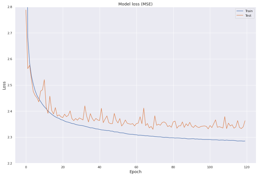
We present the model loss (mean squared error) values for both the effective training set and the validation set in the last fifteen epochs.
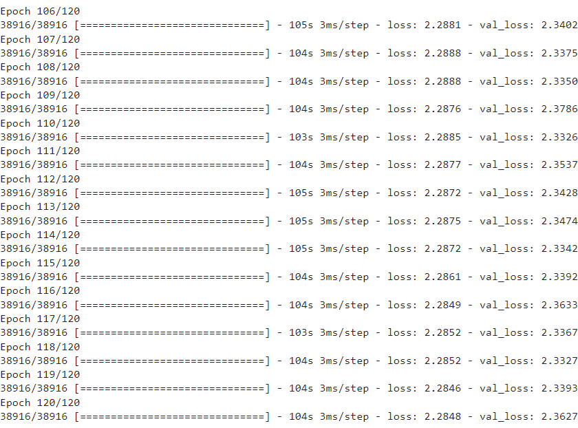
We plot the model loss for both the effective training set and the validation set against the epochs.
Model Evaluation
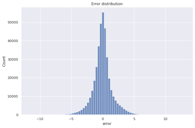
We use the fitted model to predict on the training set and the test set. The error distribution for prediction of ELE_TOTAL_ENERGY_FLUX_LOG in the test set is shown below.
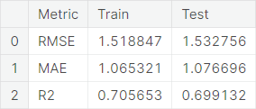
We summarize the baseline model performance through the evaluation metrics RMSE, MAE, and \(R^2\).
○ Hyperparameter Tuning
In this project, we tune the number of units in the first dense layer and the learning rate for the optimizer using the KerasTuner library.
Model Builder
The next function builds a model, with specified set of values for the hyperparameters to be optimized.
def model_builder(hp):
    model = Sequential()
    model.add(Flatten(input_shape = (X_train.shape[1],)))

    hp_units = hp.Int('units', min_value = 128, max_value = 512, step = 128)
    model.add(Dense(units = hp_units, activation = 'relu'))
    model.add(Dense(units = 64, activation = 'relu'))
    model.add(Dense(units = 32, activation = 'relu'))
    model.add(Dense(units = 16, activation = 'relu'))
    model.add(Dense(units = 4, activation = 'relu'))
    model.add(Dense(units = 1, activation = 'linear'))

    hp_learning_rate = hp.Choice('learning_rate', values = [0.01, 0.001, 0.0001])
    model.compile(loss = 'mean_squared_error', optimizer = Adam(learning_rate = hp_learning_rate))

    return model
Keras Tuner
We now make the tuner using the Hyperband function, setting the objective as validation loss.
tuner = kt.Hyperband(model_builder, objective = 'val_loss', max_epochs = 120, factor = 2, directory = 'dir_1')
We summarize the search space for the tuner.

Tuner Search
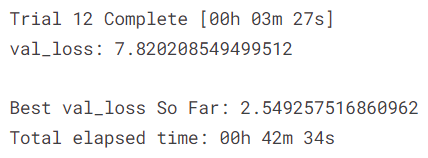
We implement the tuner using the search function.
tuner.search(X_train, y_train, epochs = 120, validation_split = 0.2)
We retrieve the optimal values of the hyperparameters to be tuned using the get_best_hyperparameters function.
hp_tuned = tuner.get_best_hyperparameters()[0]
Next, we build the model with optimal hyperparameter values.
model_tuned = tuner.hypermodel.build(hp_tuned)
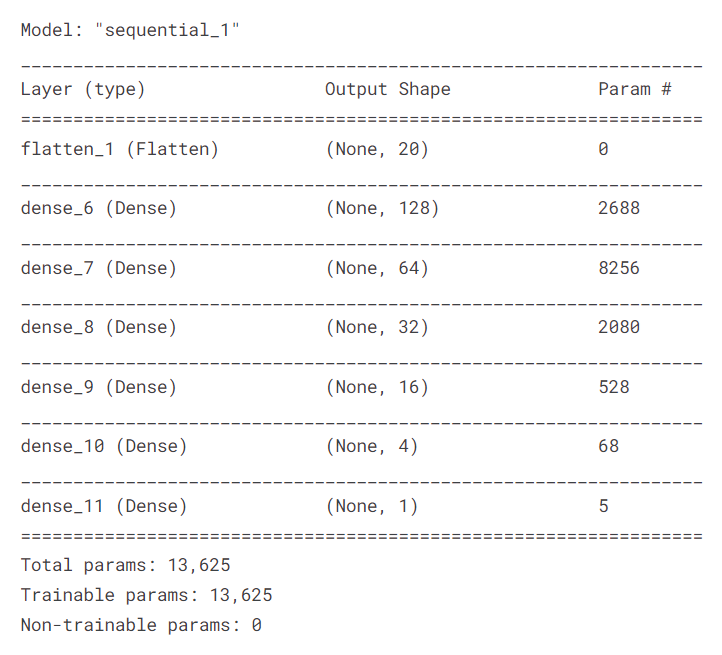
A summary of the tuned model is given below.
Tuned Model Fitting
We fit the model for \(120\)
epochs. Specifically, we set aside \(20\%\)
training samples as validation data through the argument validation_split. We train the model on the rest of the training observations (effective training set) and evaluate it on the validation data.
On the effective training set (first \(80\%\) observations from the original training set) and evaluate it on the validation set (last \(20\%\) samples from the original training set).
history_tuned = model_tuned.fit(X_train, y_train, epochs = 120, validation_split = 0.2)
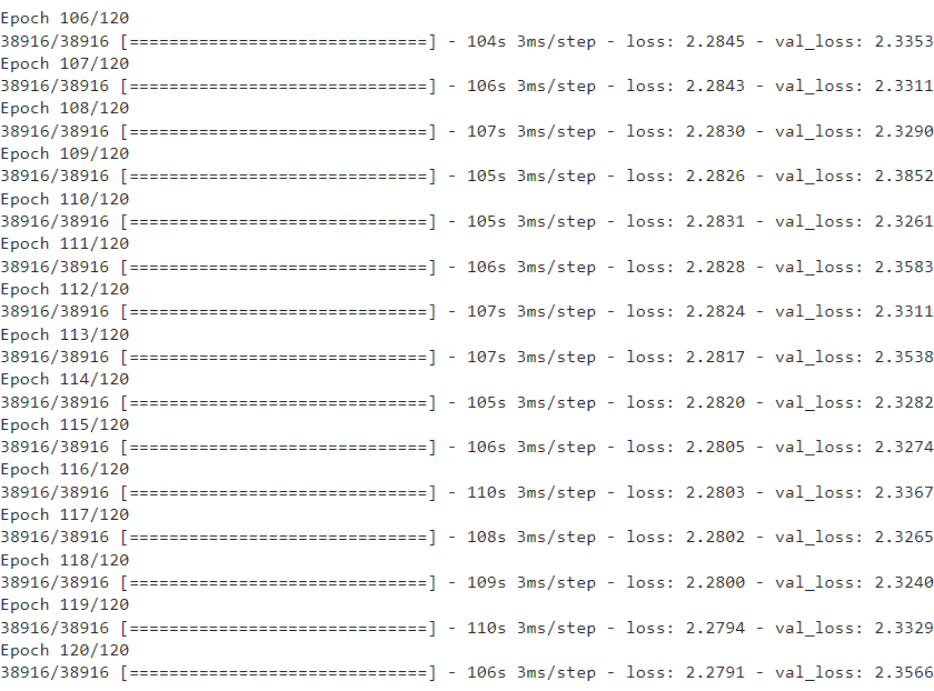
We present the model loss for both the effective training set and the validation set in the last fifteen epochs.
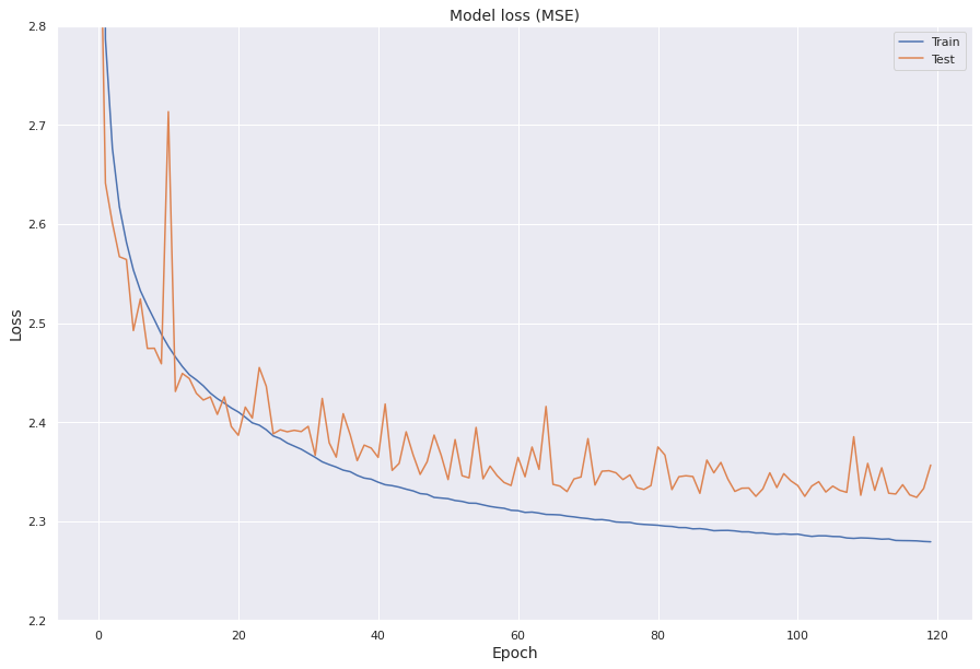
We visualize the model loss for both the effective training set and the validation set against the epochs.
○ Prediction and Evaluation
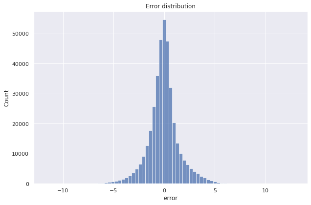
We use the fitted tuned model to predict on the training set and the test set. The error distribution for prediction of ELE_TOTAL_ENERGY_FLUX_LOG (by the tuned model) in the test set is shown below.
We summarize the hyperparameter-tuned model performance below.

Comparing with the baseline model performance, we observe that the model obtained after tuning hyperparameters performs slightly better.
○ Acknowledgements
- Toward a Next Generation Particle Precipitation Model: Mesoscale Prediction Through Machine Learning (a Case Study and Framework for Progress)
- DMSP Particle Precipitation AI-ready Data
○ References
- Activation function
- Adam optimizer
- Coefficient of determination
- Continuous variable
- Correlation coefficient
- Data leakage
- Data preprocessing
- Data transformation
- Exploratory data analysis
- Feature scaling
- Hyperparameter optimization
- Ionosphere
- KerasTuner
- Layer types
- Logarithmic scale
- Machine learning
- Magnetosphere
- Mean absolute error
- Mean squared error
- Min-max normalization
- Neural network
- Root mean square deviation
- Seaborn histplot
- Sequential model
- Stochastic gradient descent
- Test set
- Training set
- Train-test split
- Unit of measurement