Credit Card Fraud Detection
The detection of a fraudulent credit card transaction can be helped by a number of attributes regarding the particular transaction. In this work, we build a number of classification models to predict whether a credit card transaction is authentic or fraudulent based on the data regarding time, amount, and a set of PCA-transformed features. Apart from the unaltered training set, we use different resampled training sets (with both classes represented equally) to counter the class imbalance issue.
○ Contents
- Overview
- Introduction
- Exploratory Data Analysis
- Train-Test Split
- Resampling
- Feature Scaling
- Baseline Models
- Conclusion
- Acknowledgements
- References
○ Overview
- Detection of a fraudulent credit card transaction can be helped by a number of factors such as the time and amount of the transaction.
- In this project, we build classification models to predict whether a credit card transaction is authentic or fraudulent, based on the data regarding time, amount and a set of PCA-transformed features for a large number of transactions.
- A detailed exploratory data analysis on the dataset is carried out.
- We observe that the data is imbalanced with respect to the target variable. After splitting the data into training set and test set, we consider three undersampling and three oversampling techniques to balance the training set.
- We scale the features appropriately through a modified version of the min-max normalization.
- We employ a number of classifiers, namely logistic regression, \(k\)-nearest neighbors classifier, decision tree, support vector machine with linear kernel, naive Bayes classifier, random forest, linear discriminant analysis, stochastic gradient descent, and ridge classifier.
- The performance of these classifiers, trained separately on the unaltered training set as well as the training set obtained from each of the six resampling approaches, are evaluated through a number of evaluation metrics. Considering the nature of the problem, we use \(F_2\)-score as the primary metric to evaluate the models.
- The random forest algorithm applied on the training set obtained after oversampling the minority class (fraudulent transactions) via synthetic minority over-sampling technique (SMOTE) appears to perform best, in terms of \(F_2\)-score, on the test set. It achieves a test \(F_2\)-score of \(0.880783\).
- The best model with the optimal resampling scheme, stated above, has the following confusion matrix, depicting its performance on the test set.

○ Introduction
The ability to detect fraudulent transactions is of critical importance to all credit card companies. In this project, we classify credit card transactions as authentic or fraudulent based on the data regarding time, amount and a set of PCA-transformed features for a large number of transactions. We explore the data extensively and employ different techniques to build classification models, which are compared through various evaluation metrics.
Data
The dataset contains information on the transactions made using credit cards by European cardholders in two particular days of September, \(2013\). It presents a total of \(284807\) transactions, of which \(492\) were fraudulent.
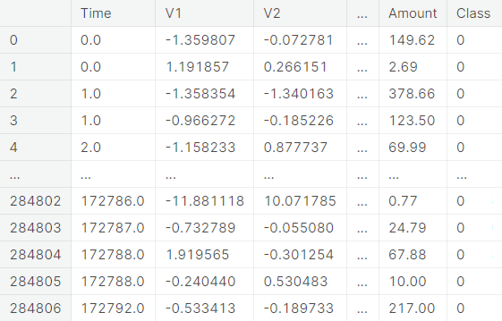
For a particular transaction, the feature Time represents the time (in seconds) elapsed between the transaction and the very first transaction, Amount represents the amount of the transaction and Class represents the status of the transaction with respect to authenticity. The class of an authentic (resp. fraudulent) transaction is taken to be \(0\)
(resp. \(1\)).
Rest of the variables (V\(1\)
to V\(28\))
are obtained from PCA-transformation on original features that are not available due to confidentiality.
Project Objective
The aim of the project is to build models based on relevant data regarding a credit card transaction, such as time, amount, and a set of PCA-transformed features, to classify the transactions into the following two classes:
- Authentic transaction
- Fraudulent transaction
Thus, it is a binary classification problem.
Evaluation Metric
Let us denote
- TP: Number of true positives
- TN: Number of true negatives
- FP: Number of false positives
- FN: Number of false negatives
We shall see in the next section that the data is highly imbalanced with respect to the target variable Class. For this reason, we do not give much importance to the accuracy metric, given as
in this project as it produces misleading conclusion when the classes are not balanced. Precision and recall are universally accepted metrics to capture the performance of a model, when restricted respectively to the predicted positive class and the actual positive class. These metrics are defined as
The \(F_1\)-score provides a balanced measuring stick by considering the harmonic mean of the above two metrics.
For its equal emphasis on both precision and recall, \(F_1\)-score is one of the decent metrics for evaluating the models in this project. The weightage between precision and recall in this metric can be parametrized, leading to the generalized notion of \(F_{\beta}\)-score , given as
Another good choice of evaluation metric, in particular for imbalanced dataset, is Matthews Correlation Coefficient (MCC), given as
The MCC metric is symmetric with respect to class, i.e. if one relabels the positive class as negative and the negative class as positive, the metric remains the same. In the problem at hand, however, the positive class is more critical than the negative class. Thus, such relabeling should change the metric used for evaluation.
To elaborate, in the context of this particular problem, false negative (a fraudulent transaction being classified as authentic) is more dangerous than false positive (an authentic transaction being classified as fraudulent) as in the former case, the fraudster can cause further financial damage, while in the latter case the bank can cross-verify the authenticity of the transaction from the card-user after taking necessary steps to secure the card.
Considering this fact, we give recall twice as more importance as precision and choose \(F_2\)-score as the primary metric to evaluate the models in this project. It is obtained by setting \(\beta = 2\) in \(F_{\beta}\)-score.
○ Exploratory Data Analysis
Visualizing individual features
First we analyze the feature which is the main object of the study: the target variable Class, which indicates if a particular transaction is authentic or fraudulent.
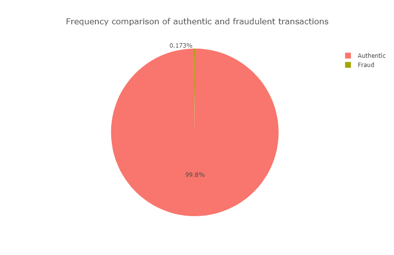
It is evident that the data is extremely imbalanced in terms of the target variable Class. It turns out that the negative class (authentic transactions) is the majority class and the positive class (fraudulent transactions) is the minority class. To be specific, the positive class accounts for only \(0.173\%\)
of all transactions.
Next, we analyze the frequency of transactions made over time elapsed starting from the first transaction.
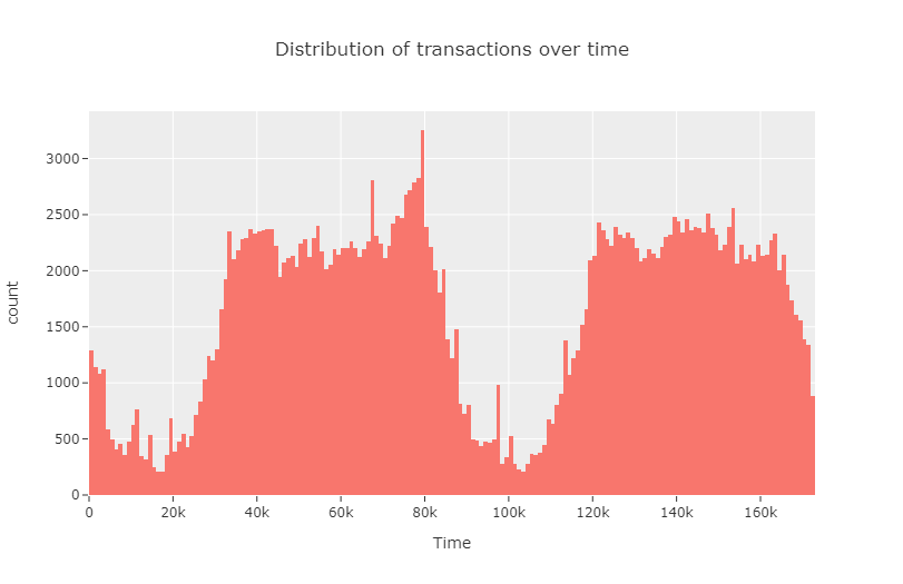
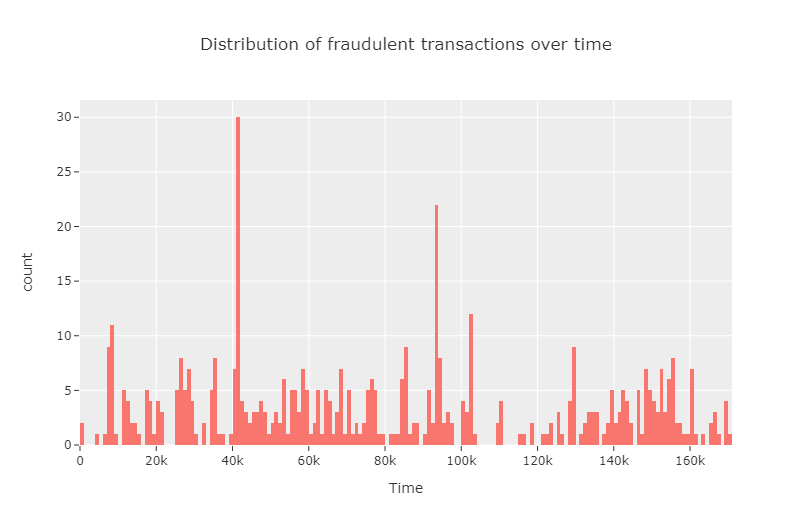
We observe that the number of transactions are particularly high in certain time intervals and low in between. Next, we analyze the same, focusing only on the fraudulent transactions.
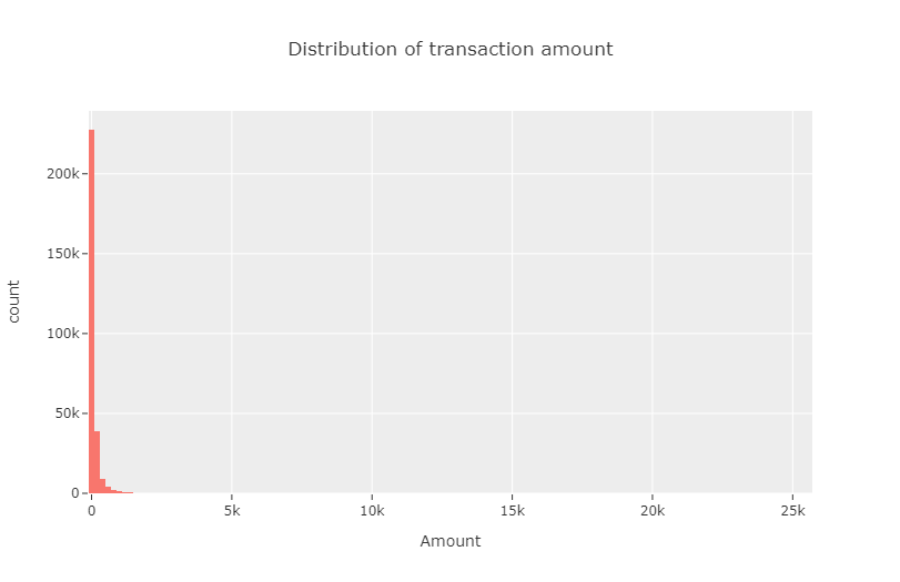
Next, we visualize the distribution of transaction amount. It is seen from the data that this feature is positively skewed to a great extent. Hence, we use logarithmic scale in the \(y\)-axis to produce a nondegenerate visualization of the same.
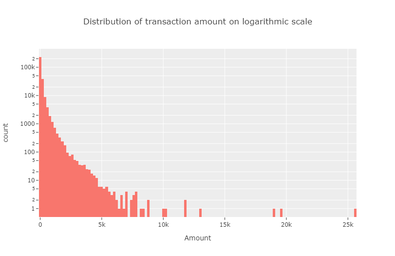
The high positive skewness even after taking the logarithmic scale motivates us to map the amount data using log transformation.
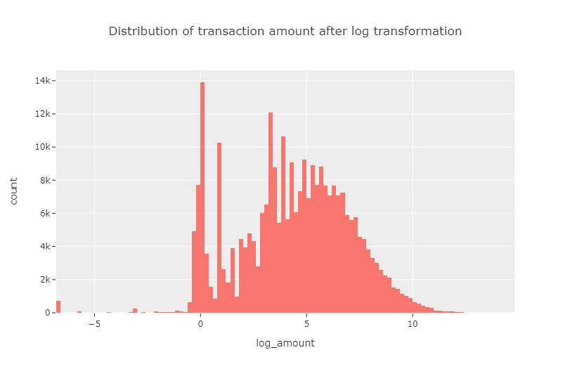
Since this gives a more symmetric output, we are motivated to work with this transformed amount data, from which the original amount data can easily be converted back to.
Next, we visualize the distributions of the log-transformed amount of authentic and fraudulent transactions.

It is clear from the plots that most of the large-amount transactions are authentic, which maybe caused by the extra security measures given to high-amount transactions in form of multiple passwords and OTPs.
For visualizations of the distributions of the PCA-transformed variables V\(1\) to V\(28\), see this notebook.
Relationships among the features
First, we analyze how the amount of transaction behaves with respect to time.
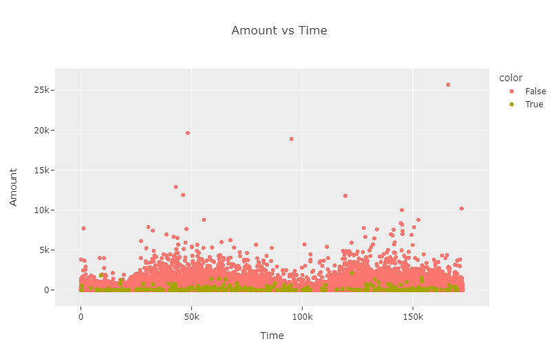
We split up the scatterplot into two different subplots, one for authentic transactions and the other for fraudulent transactions.
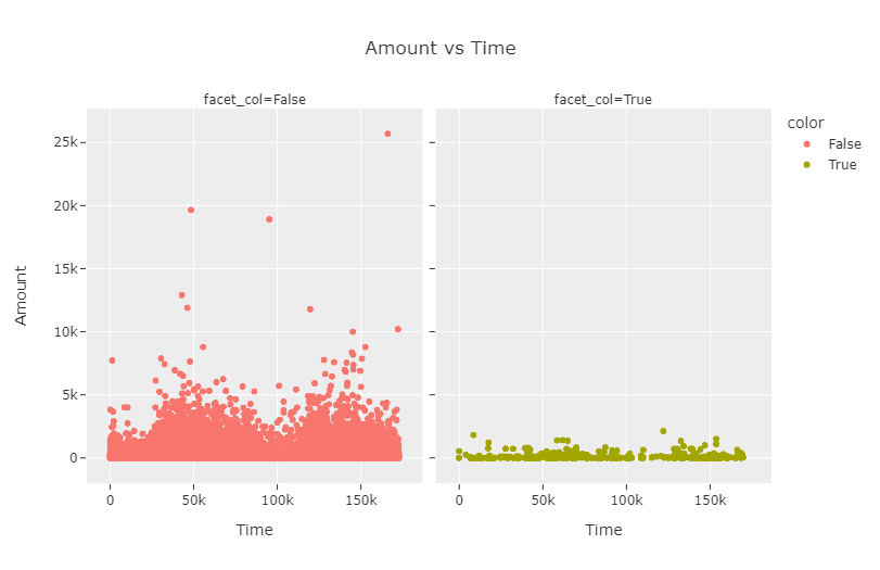
Note that facet_col=False corresponds to the authentic transactions and facet_col=True corresponds to the fraudulent transactions. We zoom into the second subplot a bit to get a clearer picture.
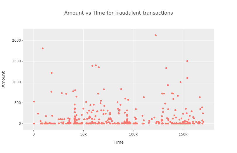
We compute the correlation coefficient between Time and Amount. The two features appear to be approximately uncorrelated, which is echoed even when the authentic transactions and the fraudulent transactions are considered separately.

In this notebook, we take the analysis further by examining bivariate scatterplots and linear relationships between certain pairs of feature variables, which exhibit contrasting correlation structures for authentic and fraudulent transactions.
○ Train-Test Split
First, we separate out the target variable from the features using the following function.
def predictor_target_split(data, target):
    X = data.drop(target, axis = 1)
    y = data[target]
    return X, y
We split the dataset into training set and test set in \(80 : 20\) ratio.
X_train, X_test, y_train, y_test = train_test_split(X, y, test_size = 0.2, random_state = 25)
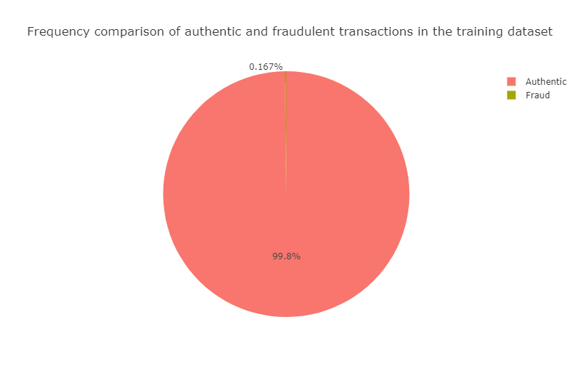
The fraudulent transactions make up for only \(0.167\%\) of the training set. Thus we run into the risk of training models with a representative sample of fraudulent transactions of extremely small size.
○ Resampling
- Random under-sampling
- Random over-sampling
- Random under-sampling with imbalanced-learn library
- Random over-sampling with imbalanced-learn library
- Synthetic minority over-sampling technique (SMOTE)
- Under-sampling via NearMiss
We start with two basic approaches based on random sampling. First, we define a function to split the dataset by the target variable Class.
def split_by_target(data):
    authentic = data[data['Class'] == 0]
    fraudulent = data[data['Class'] == 1]
    return authentic, fraudulent
Random under-sampling
Here the number of authentic observations is more than the number of fraudulent observations. In random under-sampling (RUS), we under-sample the class of authentic observations so that the size of the two classes become equal.
def rus(X_train, y_train):
    train = pd.concat([X_train, y_train], axis = 1)
    authentic, fraudulent = split_by_target(train)
    authentic_rus = authentic.sample(len(fraudulent))
    train_rus = pd.concat([authentic_rus, fraudulent], axis = 0)
    X_train_rus, y_train_rus = predictor_target_split(train_rus, 'Class')
    return X_train_rus, y_train_rus
Random over-sampling
In random over-sampling (ROS), we over-sample the class of fraudulent observations so that the size of the two classes become equal. Note that by setting replace = True, we employ sampling with replacement, so that a single observation can be sampled more than once.
def ros(X_train, y_train):
    train = pd.concat([X_train, y_train], axis = 1)
    authentic, fraudulent = split_by_target(train)
    fraudulent_ros = authentic.sample(len(authentic), replace = True)
    train_ros = pd.concat([authentic, fraudulent_ros], axis = 0)
    X_train_ros, y_train_ros = predictor_target_split(train_ros, 'Class')
    return X_train_ros, y_train_ros
The next methods make use of the imbalanced-learn library, imported as imblearn. It is an open source, MIT-licensed library relying on the scikit-learn library, imported as sklearn. It provides tools for dealing with classification with imbalanced classes.
To implement these methods, we import the relevant class from the imbalanced-learn library. We then fit an instance of the class (object) on the training set and resample it to obtain the desired version of the training set with both the authentic transactions and the fraudulent transactions represented equally.
Random under-sampling with imbalanced-learn library
The following function implements random under-sampling with imbalanced-learn library (RUS-IL).
def rusil(X_train, y_train):
    rusil_ = RandomUnderSampler(random_state = 40, replacement = True)
    X_train_rusil, y_train_rusil = rusil_.fit_resample(X_train, y_train)

    X_train_rusil = pd.DataFrame(X_train_rusil, columns = X_train.columns)
    y_train_rusil = pd.DataFrame(y_train_rusil, columns = ['Class'])
    train_rusil = pd.concat([X_train_rusil, y_train_rusil], axis = 1)
    X_train_rusil, y_train_rusil = predictor_target_split(train_rusil, 'Class')

    return X_train_rusil, y_train_rusil
Random over-sampling with imbalanced-learn library
The next function implements random over-sampling with imbalanced-learn library (ROS-IL).
def rosil(X_train, y_train):
    rosil_ = RandomOverSampler(random_state = 40)
    X_train_rosil, y_train_rosil = rosil_.fit_resample(X_train, y_train)

    X_train_rosil = pd.DataFrame(X_train_rosil, columns = X_train.columns)
    y_train_rosil = pd.DataFrame(y_train_rosil, columns = ['Class'])
    train_rosil = pd.concat([X_train_rosil, y_train_rosil], axis = 1)
    X_train_rosil, y_train_rosil = predictor_target_split(train_rosil, 'Class')

    return X_train_rosil, y_train_rosil
Synthetic minority over-sampling technique (SMOTE)
The following function implements synthetic minority over-sampling technique (SMOTE).
def smote(X_train, y_train):
    smote_ = SMOTE()
    X_train_smote, y_train_smote = smote_.fit_resample(X_train, y_train)

    X_train_smote = pd.DataFrame(X_train_smote, columns = X_train.columns)
    y_train_smote = pd.DataFrame(y_train_smote, columns = ['Class'])
    train_smote = pd.concat([X_train_smote, y_train_smote], axis = 1)
    X_train_smote, y_train_smote = predictor_target_split(train_smote, 'Class')

    return X_train_smote, y_train_smote
Under-sampling via NearMiss
The next function implements under-sampling via NearMiss (NM).
def nm(X_train, y_train):
    nm_ = NearMiss()
    X_train_nm, y_train_nm = nm_.fit_resample(X_train, y_train)

    X_train_nm = pd.DataFrame(X_train_nm, columns = X_train.columns)
    y_train_nm = pd.DataFrame(y_train_nm, columns = ['Class'])
    train_nm = pd.concat([X_train_nm, y_train_nm], axis = 1)
    X_train_nm, y_train_nm = predictor_target_split(train_nm, 'Class')

    return X_train_nm, y_train_nm
○ Feature Scaling
It may be natural for one of the features to contribute to the classification process more than another. But often this is caused artificially by the difference of range of values that the features take (often due to the units in which the features are measured). Many algorithms, especially the tree-based ones like decision tree and random forest, as well as graphical model-based classifiers like linear discriminant analysis and naive Bayes classifier, are invariant to scaling and hence indifferent to feature scaling. On the other hand, algorithms based on distances or similarities, such as \(k\)-nearest neighbours classifier, support vector machine, and stochastic gradient descent, are sensitive to scaling. This necessitates the practitioner to scale the features appropriately before feeding the data to such classifiers. For this purpose, the min-max normalization transforms the features in the following way:
In this project, we modify the scaling so that the feature values are mapped to the range \([-1, 1].\)
This is done by mapping the above quantity by \(y \mapsto 2y - 1.\)
We implement this using the MinMaxScaler class from the scikit-learn library, setting the feature_range argument to \((-1, 1).\)
To keep the transformation the same, we use the minimum and maximum values of the training columns only for both DataFrames. Using the minimum and maximum values of the test columns for both sets would have led to data leakage. Specifically, we use \(\min{\left(x\right)}\) and \(\max{\left(x\right)}\) for a particular feature from the training set to rescale the feature for both the training set and the test set.
def scaler(X_train, X_test):
    scaling = MinMaxScaler(feature_range = (-1, 1)).fit(X_train)
    X_train_scaled = scaling.transform(X_train)
    X_test_scaled = scaling.transform(X_test)
    return X_train_scaled, X_test_scaled
○ Baseline Models
- Logistic Regression
- k-Nearest Neighbors
- Decision Tree
- Support Vector Machine
- Naive Bayes
- Random Forest
- Linear Discriminant Analysis
- Stochastic Gradient Descent
- Ridge Classifier
- Summary of the Baseline Models
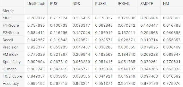
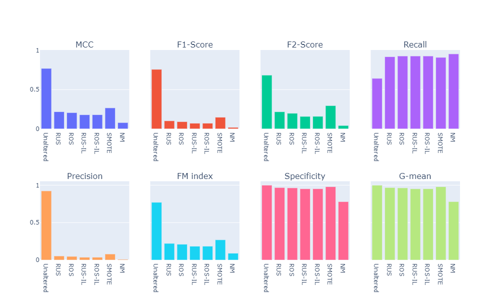
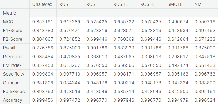
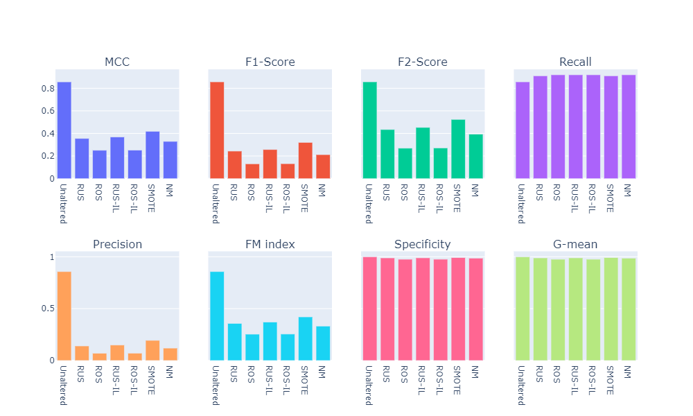
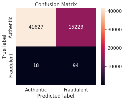
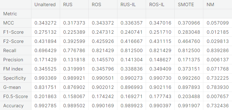
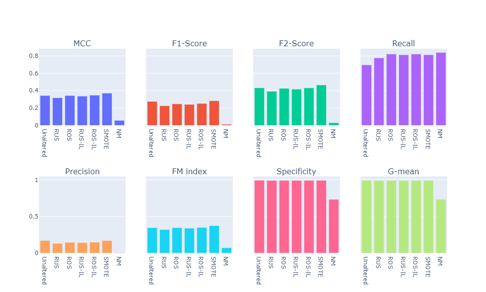
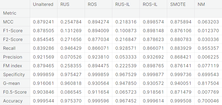
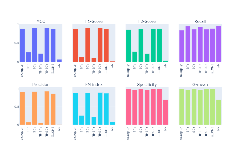
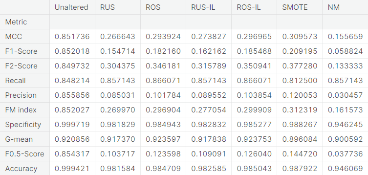
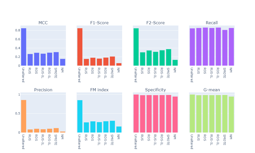
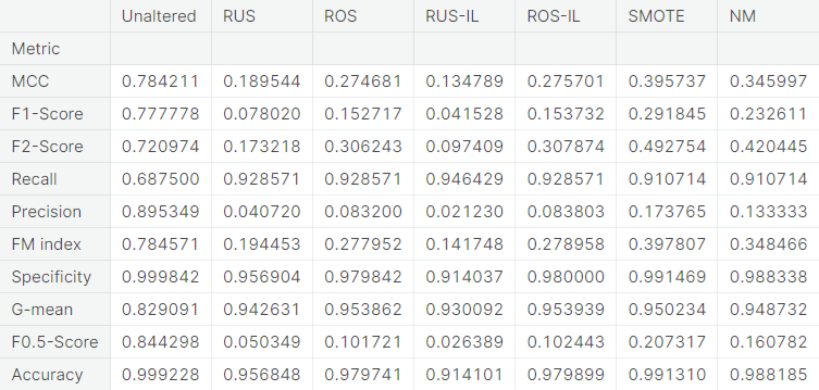
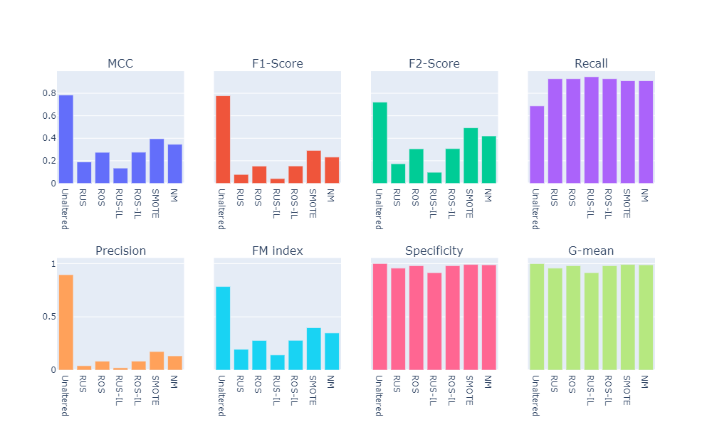
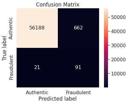
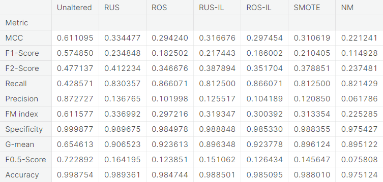
We consider a number of binary classifiers and train each of them on the original training set as well as the training sets obtained from different resampling approaches. In each case, the confusion matrix depicting the test set performance is reported. The computed values of several relevant evaluation metrics are summarized in tabulated form. Additionally, we compare the resampling approaches for each classifier visually.
For the sake of brevity, we omit the code snippets for computation of confusion matrix, evaluation metrics, and visualization of classes. The codes can be found in this notebook.
Logistic Regression
- Unaltered training set
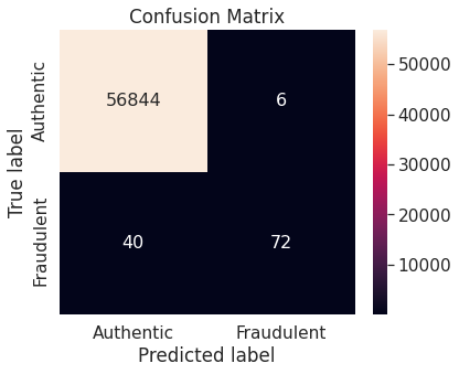

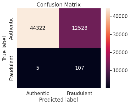
Logistic regression model on unaltered training set performs very well on the negative class (authentic transactions). However, it does not work so well with the critical positive class (fraudulent transactions) as it misclassifies more than one-third of the transactions in that class.
- Random under-sampling


Note that the resampling approach immediately brings down the proportion of misclassified observations in the positive class, though at the expense of a slight increase in the same in the negative class.
- Random over-sampling


- Random under-sampling with imbalanced-learn library


- Random over-sampling with imbalanced-learn library


- Synthetic minority over-sampling technique (SMOTE)


- Under-sampling via NearMiss

- Numerical summary
- Visual summary
k-Nearest Neighbors
- Unaltered training set


- Random under-sampling


- Random over-sampling


- Random under-sampling with imbalanced-learn library


- Random over-sampling with imbalanced-learn library


- Synthetic minority over-sampling technique (SMOTE)


- Under-sampling via NearMiss


- Numerical summary
- Visual summary
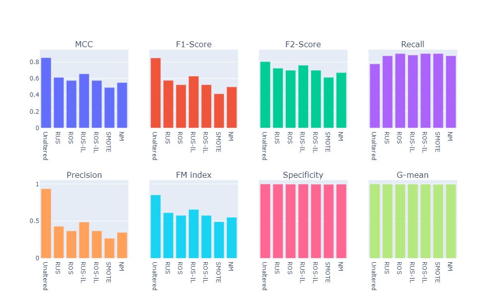
A potential issue with KNN classification model, which is relevant in this project, is that they are affected by the curse of dimensionality as well as the presence of outliers in the feature variables. Despite that, it performs fairly well when applied to the unaltered (imbalanced) training set.
Decision Tree
- Unaltered training set


- Random under-sampling

- Random over-sampling


- Random under-sampling with imbalanced-learn library


- Random over-sampling with imbalanced-learn library


- Synthetic minority over-sampling technique (SMOTE)


- Under-sampling via NearMiss

- Numerical summary

- Visual summary

Support Vector Machine
- Unaltered training set


- Random under-sampling


- Random over-sampling


- Random under-sampling with imbalanced-learn library


- Random over-sampling with imbalanced-learn library


- Synthetic minority over-sampling technique (SMOTE)


- Under-sampling via NearMiss


- Numerical summary
- Visual summary
Naive Bayes
- Unaltered training set


- Random under-sampling


- Random over-sampling


- Random under-sampling with imbalanced-learn library


- Random over-sampling with imbalanced-learn library


- Synthetic minority over-sampling technique (SMOTE)


- Under-sampling via NearMiss

- Numerical summary
- Visual summary
Random Forest
The Random Forest classifier employs multiple decision trees, thereby avoiding the reliance upon feature selection of a singular decision tree.
- Unaltered training set


- Random under-sampling


- Random over-sampling


- Random under-sampling with imbalanced-learn library


- Random over-sampling with imbalanced-learn library


- Synthetic minority over-sampling technique (SMOTE)


- Under-sampling via NearMiss


- Numerical summary
- Visual summary
Linear Discriminant Analysis
- Unaltered training set


- Random under-sampling


- Random over-sampling


- Random under-sampling with imbalanced-learn library


- Random over-sampling with imbalanced-learn library


- Synthetic minority over-sampling technique (SMOTE)


- Under-sampling via NearMiss


- Numerical summary
- Visual summary
Stochastic Gradient Descent
- Unaltered training set


- Random under-sampling


- Random over-sampling


- Random under-sampling with imbalanced-learn library

- Random over-sampling with imbalanced-learn library


- Synthetic minority over-sampling technique (SMOTE)


- Under-sampling via NearMiss


- Numerical summary
- Visual summary
Ridge Classifier
- Unaltered training set


- Random under-sampling


- Random over-sampling


- Random under-sampling with imbalanced-learn library


- Random over-sampling with imbalanced-learn library


- Synthetic minority over-sampling technique (SMOTE)

- Under-sampling via NearMiss


Summary of the Baseline Models
- Numerical summary
- Visual summary

○ Conclusion
For each classifier, we choose the resampling approach which gives the highest \(F_2\)-score. The next table summarizes the test set performance of different classifiers, acting on the chosen resampled (or unaltered) dataset, ranked by \(F_2\)-score. Additionally, we report MCC and recall.
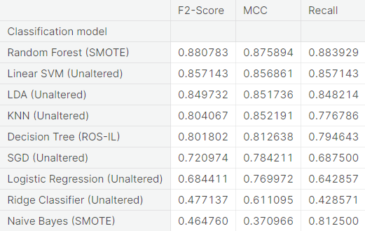
The Random Forest algorithm applied on the training set obtained after oversampling the minority class (fraudulent transactions) via SMOTE appears to perform best, in terms of \(F_2\)-score, for the problem at hand. We restate the confusion matrix, which depicts the test set performance of this model under the particular resampling approach.

SMOTE is one of the best choices to oversample the minority class when the data is imbalanced. It is not surprising that Random Forest turns out to be one of the most suitable classifiers for the problem due to the following reasons:
- The algorithm works well in dealing with large datasets with high dimensions.
- It is less affected by the presence of outliers in feature variables compared to other algorithms.
- It does not make any distributional assumption on the feature variables.
- It handles collinearity (linear dependence among features) implicitly.
- It automatically ignores the features which are not useful, effectively doing feature selection on its own.
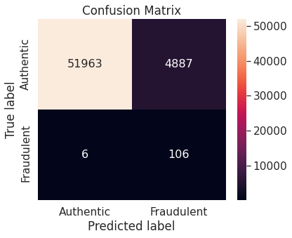
Many other (classifier + resampling approach) combinations produce better test set performance on the critical positive class compared to (Random Forest + SMOTE). However, as a trade-off, the decrease in the performance on the negative class can be significant. For example, we refer to the confusion matrices depicting the test set performance of logistic regression, support vector machine, and stochastic gradient descent classifier acting on any of the resampled training set (but not the unaltered training set).
○ Acknowledgements
○ References
- Accuracy
- Binary classification
- Classification
- Confusion matrix
- Credit card
- Curse of dimensionality
- Data leakage
- Decision tree
- Evaluation metric
- Exploratory data analysis
- False negative
- False positive
- Feature scaling
- \(F\)-score
- Imbalanced-learn library
- \(k\)-nearest neighbors algorithm
- linear discriminant analysis
- Logarithm
- Logarithmic scale
- Logistic regression
- Matthews correlation coefficient
- Min-max normalization
- Naive Bayes classifier
- NearMiss
- Outlier
- Oversampling
- Precision
- Principal component analysis
- Random forest
- Random sampling
- Random over-sampling
- Random over-sampling with imbalanced-learn library
- Random under-sampling
- Random under-sampling with imbalanced-learn library
- Recall
- Ridge classifier
- Scikit-learn library
- Stochastic gradient descent
- Support vector machine
- Synthetic minority over-sampling technique
- Test set
- Training set
- Train-test split
- Undersampling
- Unit of measurement