Anomaly Detection in Credit Card Transactions
An anomaly or outlier refers to a rare observation that deviates significantly from the majority of the data and does not conform to a well-defined notion of normal behaviour. Anomaly detection can be very useful in identifying fraudulent credit card transactions, which are rare compared to authentic transactions. Also, the methods through which fraudulent transactions occur keep evolving as the old ways get flagged by existing fraud detection systems. In this project, we shall develop a basic anomaly detection system that flags transactions with feature values deviating significantly from those of authentic transactions.
○ Contents
- Overview
- Introduction
- Train-Validation-Test Split
- Feature Engineering
- Feature Selection
- Implementing Anomaly Detection
- Threshold Tuning on Validation Set
- Prediction and Evaluation on Test Set
- Conclusion
- Acknowledgements
- References
○ Overview
In this project, we consider an imbalanced dataset of credit card frauds (with the target labels being authentic and fraudulent) and build an anomaly detection system to identify transactions that are, in some sense, different from the usual, authentic transactions. These observations are flagged as potentially fraudulent and put to further verification.
- We carry out necessary feature extraction and feature transformation.
- As the anomaly detection algorithm suffers from high-dimensional data, we figure out the most relevant features separating the target classes, and use only those in the modeling purpose.
- Based on the training data, we fit a multivariate normal distribution.
- Given a new transaction, if the corresponding density value of the fitted distribution is lower than a pre-specified threshold, then we flag the transaction as fraudulent.
- We focus more on the true positive class (the class of fraudulent transactions) than the true negative class (the class of authentic transactions). This is because a false negative (the algorithm predicts a fraudulent transaction as authentic) is far more dangerous than a false positive (the algorithm predicts an authentic transaction as fraudulent, which can always be cross-verified). For this reason, we use \(F_2\)-score as the evaluation metric.
- The choice of the threshold is optimised by iterating over a pre-specified set of values, predicting on the validation set, and evaluating the predictions by means of the \(F_2\)-score.
- In this work, the optimal threshold value comes out to be \(0.009^9 \approx 3.87 \times 10^{-19}\).
- The corresponding \(F_2\)-score for predictions on the validation set is \(0.834671\), which is an optimistic projection due to the threshold tuning over the validation set.
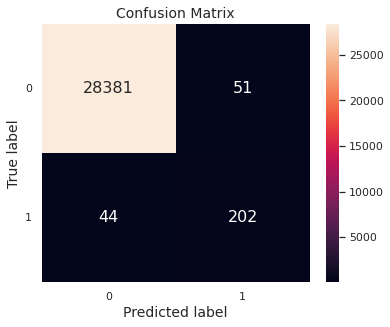
- Applying the same model on the test set, we get predictions with an \(F_2\)-score of \(0.816492\). The confusion matrix for predictions on the test set is given below.
○ Introduction
Anomaly Detection
In statistics and data analysis, an anomaly or outlier refers to a rare observation which deviates significantly from the majority of the data and does not conform to a well-defined notion of normal behaviour. It is possible that such observations may have been generated by a different mechanism or appear inconsistent with the remainder of the dataset. The process of identifying such observations is generally referred to as anomaly detection.
In recent days, machine learning is progressively being employed to automate the process of anomaly detection through supervised learning (when observations are labeled as normal or anomalous), semi-supervised learning (when only a small fraction of observations are labeled) and unsupervised learning (when observations are not labeled). Anomaly detection is particularly suitable in the following setup:
- Anomalies are very rare in the dataset
- The features of anomalous observations differ significantly from those of normal observations
- Anomalies may result for different (potentially new) reasons
Anomaly detection can be very useful in credit card fraud detection. Fraudulent transactions are rare compared to authentic transactions. Also, the methods through which fraudulent transactions occur keep evolving, as the old ways get flagged by existing fraud detection systems. In this project, we shall develop a basic anomaly detection system that flags transactions with feature values deviating significantly from those of authentic transactions.
Data
Source: https://www.kaggle.com/mlg-ulb/creditcardfraud
The dataset contains information on the transactions made using credit cards by European cardholders, in two particular days of September \(2013\). It presents a total of \(284807\) transactions, of which \(492\) were fraudulent. Clearly, the dataset is highly imbalanced, the positive class (fraudulent transactions) accounting for only \(0.173\%\) of all transactions. The columns in the dataset are as follows:
- Time: The time (in seconds) elapsed between the transaction and the very first transaction
- V\(1\) to V\(28\) : Obtained from principle component analysis (PCA) transformation on original features that are not available due to confidentiality
- Amount: The amount of the transaction
- Class: The status of the transaction with respect to authenticity. The class of an authentic (resp. fraudulent) transaction is taken to be \(0\) (resp. \(1\))

Project Objective
The objective of the project is to detect anomalies in credit card transactions. To be prcise, given the data on Time, Amount and transformed features V1 to V28, our goal is to fit a probability distribution based on authentic transactions, and then use it to correctly identify a new transaction as authentic or fraudulent. Note that the target variable plays no role in constructing the probability distribution.
Evaluation Metric
Some good choices to evaluate models for imbalanced datasets are Matthews correlation coefficient (MCC) and \(F_1\)-score . Precision and recall also give useful information. We shall not give much importance to accuracy in this project as it produces misleading conclusions when the classes are not balanced.
In the problem at hand, false negative (a fraudulent transaction being classified as authentic) is more dangerous than false positive (an authentic transaction being classified as fraudulent). In the former case, the fraudster can cause further financial damage. In the latter case, the bank can cross-verify the authenticity of the transaction from the card-user after taking necessary steps to secure the card.
Considering this fact, we employ \(F_2\)-score to tune threshold parameter and to select features in the present work. All of the mentioned metrics are reported for both the validation set and the test set.
○ Train-Validation-Test Split
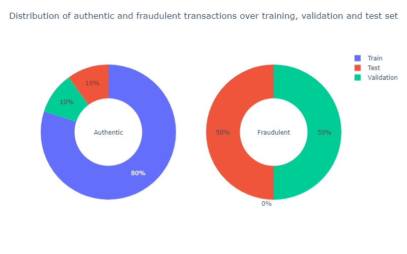
For anomaly detection, we build the classification model based on the authentic transactions only. Thus, the training set will consist entirely of authentic transactions. The validation set and the test set will have both authentic transactions and fraudulent transactions.
We split the dataset in the following way:
-
Training set \(\to\) \(80\%\) observations from the authentic class
-
Validation set \(\to\) \(10\%\) observations from the authentic class \(+\) \(50\%\) observations from the fraudulent class
-
Test set \(\to\) \(10\%\) observations from the authentic class \(+\) \(50\%\) observations from the fraudulent class
We show the distribution of authentic and fraudulent transactions over training, validation, and test set.
○ Feature Engineering
Time
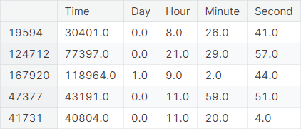
The data consists of credit card transactions on two particular days. We decompose the feature Time into the components Day, Hour, Minute, Second in the training set, the validation set, and the test set. Implementation for a specific DataFrame df:
df['Day'], temp = df['Time'] // (24*60*60), df['Time'] % (24*60*60)
df['Hour'], temp = temp // (60*60), temp % (60*60)
df['Minute'], df['Second'] = temp // 60, temp % 60
A snapshot of the new features along with the original Time feature in the training set is given below.
We visualize the distributions of the old variable Time and new variable Hour in the training set.
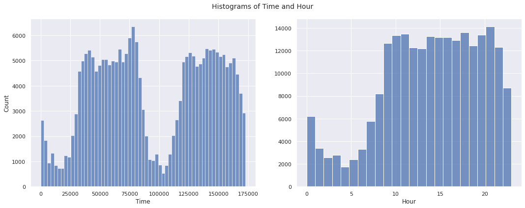
We observe a pattern of less transactions during the early hours and more transactions thereafter in the distribution of Hour. The pattern is repeated over two days in the distribution of Time.
Amount
The distribution of Amount has extreme positive skewness. We apply the transformation \(x \mapsto \log{\left(x + 0.001\right)}\)
to this column and form the new column Amount_transformed. The positive constant \(0.001\)
is added to deal with the zero-amount transactions, which leads to \(\log{0}\),
an undefined quantity. Implementation for a specific DataFrame df:
df['Amount_transformed'] = np.log10(df['Amount'] + 0.001)
We visualize the distribution of the amount of transaction before and after transformation in the training set.
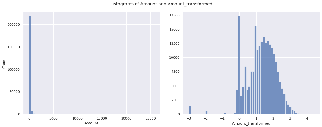
The new features Day, Minute, and Second do not influence the target variable in a meaningful way. So, we drop these features along with the old features Time and Amount. Thus, the final transformations of features are given as follows:
Time\(\mapsto\)HourAmount\(\mapsto\)Amount_transformed
○ Feature Selection
From Thudumu et al. (2020):
High dimensionality creates difficulties for anomaly detection because, when the number of attributes or features increase, the amount of data needed to generalize accurately also grows, resulting in data sparsity in which data points are more scattered and isolated. This data sparsity is due to unnecessary variables, or the high noise level of multiple irrelevant attributes, that conceal the true anomalies. This issue is widely acknowledged as the curse of dimensionality.
In the problem at hand, we have \(30\) features. We aim to keep only those which help substantially in discriminating between authentic and fraudulent transactions. For this purpose, we compare the distribution of each feature for both the target classes.
If a feature has similar distributions for both authentic and fraudulent transactions, then it is not likely to contribute much in the process of classifying a transaction as authentic or fraudulent. However, if a feature has very different distributions for different target classes, then it plays a far more significant role in the same process.
We plot the distributions of the features for the two target classes.
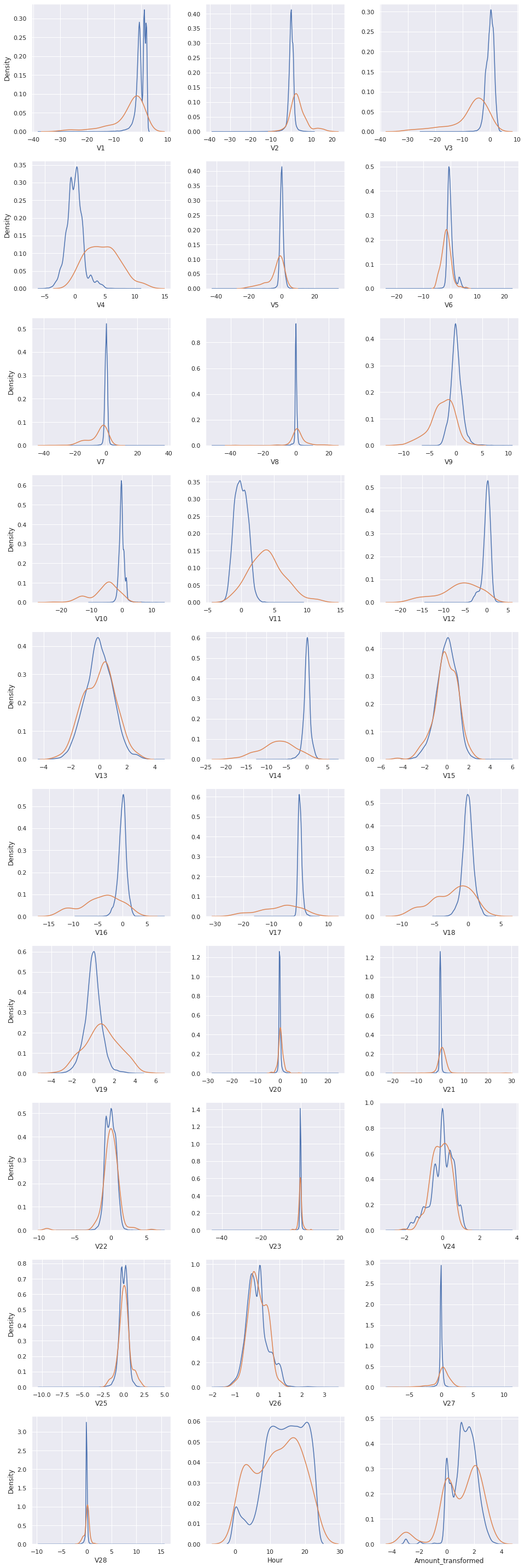
We select the features exhibiting fairly distinct distributions across the target classes. The selected features are V4, V11, V12, V14, V16, V17, V18, V19, and Hour.
We discard the other features in the training set, validation set, and test set. A snapshot of the training set after feature selection:

○ Implementing Anomaly Detection
The probability density function (pdf) of a univariate normal distribution with mean \(\mu\) and standard deviation \(\sigma\) is given by
for \(x \in \mathbb{R}\), where \(\mu \in \mathbb{R}\) and \(\sigma > 0\).
The product of such univariate normal densities can be seen as the joint pdf of a number of feature variables, each of which has a univariate normal distribution and is statistically independent of the other features.
for \(\boldsymbol{x} = \left(x_1, x_2, \cdots, x_n\right) \in \mathbb{R}^n\), where \(\boldsymbol{\mu} = \left(\mu_1, \mu_2, \cdots, \mu_n\right) \in \mathbb{R}^n\) and \(\boldsymbol{\sigma} = \left(\sigma_1, \sigma_2, \cdots, \sigma_n\right) \in (0, \infty)^n\).
We compute the vector of means and the vector of standard deviations for the features in the training set. These estimates characterize the joint probability density function of the features, which will be used to detect anomalous observations.
Then, we predict anomaly based on a given threshold \(\epsilon\) for probability density in the following way:
○ Threshold Tuning on Validation Set
We set a sequence of threshold values alpha: \(0.001, 0.002, \cdots, 0.05\).
These values are for the pdf of a single feature. The corresponding threshold for the joint probability density is alpha to the \(n\)-th
power, where \(n\)
is the number of features used in the model.
For each threshold, we compute the \(F_2\)-score
to evaluate the model performance on the validation set. The validation \(F_2\)-score
is plotted against the threshold alpha.
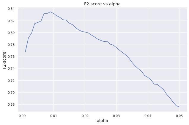
The summary of the tuning procedure is given below.

We show the confusion matrix for predictions on the validation set.

○ Prediction and Evaluation on Test Set
We predict on the test set and evaluate the performance through various evaluation metrics.
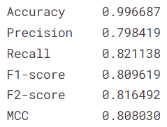
The confusion matrix for predictions on the test set is given below.

○ Conclusion
To sum up, we observed that the data is heavily imbalanced with fraudulent transaction occurring rarely compared to authentic transactions. Also there are possibilities for fraudulent transactions to occur in completely new ways than before, making it difficult to train data on fraudulent transactions. Thus we build an anomaly detection system to find transactions, which are, in some sense, different from the usual observations.
Specifically, we have extracted Hour out of the Time feature and log-transformed (with a slight shift) the highly skewed Amount feature into Amount_transformed. Out of the \(30\)
features (obtained after feature engineering), we have selected \(9\)
features which have significantly different distributions, for the different target classes: V4, V11, V12, V14, V16, V17, V18, V19 and Hour.
Based on the training data, we fit a multivariate normal distribution (by estimating the vector of means and the vector of standard deviations, assuming statistical independence among the features, which is a reasonable condition as most of the features in the provided dataset are already PCA-engineered).
Given a new transaction, if the corresponding density value of the fitted distribution is lower than a pre-specified threshold, then we flag the transaction as fraudulent. The choice of the threshold is optimized by iterating over a pre-specified set of values, predicting on the validation set, and evaluating the estimates by means of the \(F_2\)-score.
In this work, the optimal threshold value turns out to be \(0.009^9 \approx 3.87 \times 10^{-19}\). The corresponding \(F_2\)-score for predictions on the validation set is \(0.834671\), which is an optimistic projection due to the threshold tuning over the validation set. Applying the same model on the test set, we get predictions with an \(F_2\)-score of \(0.816492\).
○ Acknowledgements
- A comprehensive survey of anomaly detection techniques for high dimensional big data
- Credit Card Fraud Detection dataset
○ References
- Accuracy
- Anomaly
- Anomaly detection
- Credit card frauds
- Data analysis
- Evaluation metric
- \(F\)-score
- Fowlkes-Mallows index
- Freedman-Diaconis rule
- Labeled data
- Machine learning
- Matthews correlation coefficient
- Multivariate normal distribution
- Outlier
- Precision
- Principal component analysis
- Probability density function
- Probability distribution
- Recall
- Semi-supervised learning
- Statistics
- Supervised learning
- Test set
- Training set
- Unsupervised learning
- Validation set