Implementing Neural Network with Callbacks
A callback is an object that can perform certain actions at various stages of training. It is typically used to confirm or adjust specific behaviors and is called periodically throughout a procedure. Callbacks can be used in machine learning to specify what occurs before, during, or after a training epoch or a single batch. In this note, we implement EarlyStopping, LearningRateScheduler, and ModelCheckpoint callbacks in the training of a neural network.
○ Contents
- Data
- Visualization
- Feature Unrolling
- Target Encoding
- Model Creation
- Model Compilation
- EarlyStopping Callback
- LearningRateScheduler Callback
- ModelCheckpoint Callback
- Training
- Inference
- Evaluation
- References
○ Data
In this note, we use the MNIST dataset and consider the problem of recognizing handwritten digits. There are multiple ways to load the dataset. The keras.datasets module provides it readily.
from keras.datasets import mnist
data = mnist.load_data()
A good place to understand the data is the Keras documentation on it. Taking a quick look at the documentation page, we understand that the loaded data contains sixty thousand \(28 \times 28\) grayscale images of the \(10\) digits, along with a test set of ten thousand images.
We also see from the documentation that the data is in the format of a tuple of NumPy arrays: (X_train, y_train), (X_test, y_test).
(X_train, y_train), (X_test, y_test) = data
We check the shape of the arrays.

○ Visualization
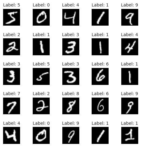
To visualize the handwritten digits from the raw data, we use the imshow function from the matplotlib.pyplot module.
import matplotlib.pyplot as plt
num_images = 25
fig, axes = plt.subplots(5, 5, figsize = (5, 5))
axes = axes.flatten()
for i in range(num_images):
    axes[i].imshow(X_train[i], cmap = 'gray')
    axes[i].axis('off')
    axes[i].set_title(f"Label: {y_train[i]}", fontsize = 10)
plt.tight_layout()
plt.show()
○ Feature Unrolling
To train a neural network on the data, we need to unroll the pixel values to a one-dimensional array. For this reason, we reshape X_train and X_test such that the \(28 \times 28\)
greyscale pixel values corresponding to each observation becomes an array of \(784\)
values.
import numpy as np
X_train_unrolled = X_train.reshape(X_train.shape[0], np.prod(X_train.shape[1:]))
X_test_unrolled = X_test.reshape(X_test.shape[0], np.prod(X_test.shape[1:]))
We check the shape of X_train_unrolled and X_test_unrolled.

○ Target Encoding
The target variable can assume \(10\) different labels. To train a neural network, we need one-hot encode it.
def vec_to_mat(y_in, num_classes = None, dtype = 'float32'):
    y_in = np.array(y_in, dtype = 'int')
    if not num_classes:
        num_classes = np.max(y_in) + 1
    m = y_in.shape[0]
    Y_out = np.zeros((m, num_classes), dtype = dtype)
    Y_out[np.arange(m), y_in] = 1
    return Y_out

Y_train_arr = vec_to_mat(y_train, num_classes = 10, dtype = 'int')
Y_test_arr = vec_to_mat(y_test, num_classes = 10, dtype = 'int')
We check the shape of Y_train_arr and Y_test_arr.

○ Model Creation
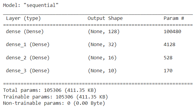
We begin by adding dense layers, with appropriate number of units and activation function, to a sequential model.
from keras.models import Sequential
from keras.layers import Dense
model = Sequential()
model.add(Dense(units = 128, input_dim = X_train_unrolled.shape[1], activation = 'relu'))
model.add(Dense(units = 32, activation = 'relu'))
model.add(Dense(units = 16, activation = 'relu'))
model.add(Dense(units = 10, activation = 'softmax'))
model.summary()
○ Model Compilation
We compile the model with binary cross-entropy loss and Adam optimizer with an input learning rate. The model is evaluated with the accuracy metric during the training process.
model.compile(
    loss = 'binary_crossentropy',
    optimizer = 'adam',
    metrics = ['accuracy']
)
Note that the Adam optimizer is set with a learning rate of \(0.001\) by default. To experiment with the learning rate parameter, we can compile the model as follows.
from keras.optimizers import Adam
model.compile(
    loss = 'binary_crossentropy',
    optimizer = Adam(learning_rate = 0.001),
    metrics = ['accuracy']
)
○ EarlyStopping Callback
The EarlyStopping callback stops the training process when a given monitored metric stops improving by a certain amount for a certain number of epochs, starting from a given epoch.
from keras.callbacks import EarlyStopping
earlystop = EarlyStopping(
    monitor = 'val_loss',
    min_delta = 0.001,
    patience = 20,
    verbose = 0,
    mode = 'auto',
    start_from_epoch = 60
)
○ LearningRateScheduler Callback
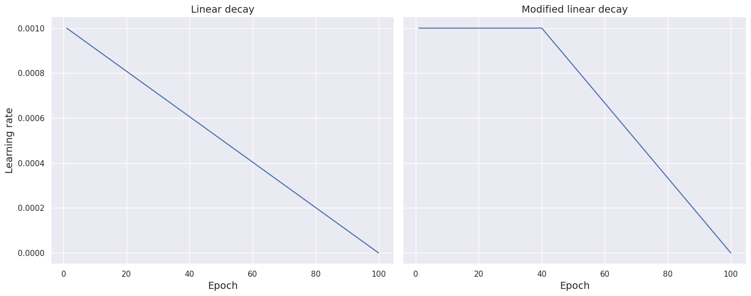
The LearningRateScheduler callback updates the learning rate value at the beginning of every epoch from an input schedule function with the current epoch and current learning rate. It then applies the updated learning rate to the optimizer.
The modified linear schedule function holds the learning rate constant for a certain number of epochs and then diminishes it linearly.
def scheduler_modified_linear(epoch, learning_rate):
    if epoch < 40:
        return learning_rate
    else:
        return learning_rate * (100 - epoch) / (100 - epoch + 1)
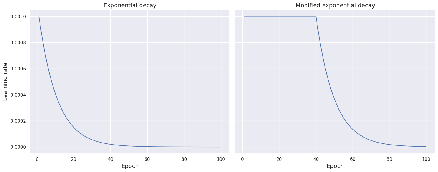
The modified exponential schedule function holds the learning rate constant for a certain number of epochs and then diminishes it exponentially.
import math
def scheduler_modified_exponential(epoch, learning_rate):
    if epoch < 40:
        return learning_rate
    else:
        return learning_rate * math.exp(-0.1)
In this note, we use the modified linear schedule function.
from keras.callbacks import LearningRateScheduler
learning_rate_scheduler = LearningRateScheduler(scheduler_modified_linear)
○ ModelCheckpoint Callback
The ModelCheckpoint callback saves the Keras model or model weights at some frequency. The model or weights can be loaded later for inference or to continue the training from the saved instance.
from keras.callbacks import ModelCheckpoint
model_checkpoint = ModelCheckpoint(
    filepath = 'best_model.h5',
    monitor = 'val_loss',
    save_best_only = True
)
○ Training
We incorporate the three callbacks in the model.fit() function and train the model on (X_train_unrolled, Y_train_arr).
history = model.fit(
    x = X_train_unrolled,
    y = Y_train_arr,
    batch_size = 32,
    epochs = 100,
    validation_split = 0.2,
    callbacks = [earlystop, learning_rate_scheduler, model_checkpoint],
    verbose = 0
)
Note: If we try to train the model on (X_train_unrolled, y_train), we would get the following error message:
ValueError: `logits` and `labels` must have the same shape, received ((32, 10) vs (32, 1)).
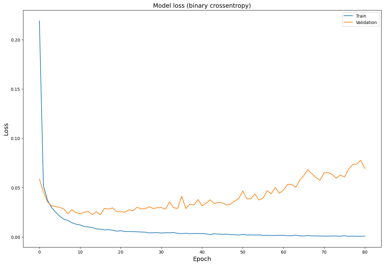
Now, we plot the model loss (binary crossentropy) against the epochs.
import seaborn as sns
plt.figure(figsize = (15, 10))
plt.title('Model loss (binary crossentropy)', fontsize = 14)
sns.lineplot(data = history.history['loss'], label = 'Train')
sns.lineplot(data = history.history['val_loss'], label = 'Validation')
plt.xlabel('Epoch', fontsize = 14)
plt.ylabel('Loss', fontsize = 14)
plt.legend()
plt.show()
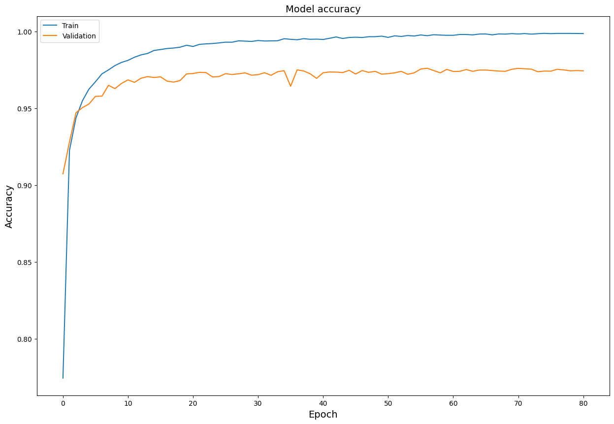
We also plot the model accuracy against the epochs.
plt.figure(figsize = (15, 10))
plt.title('Model accuracy', fontsize = 14)
sns.lineplot(data = history.history['accuracy'], label = 'Train')
sns.lineplot(data = history.history['val_accuracy'], label = 'Validation')
plt.xlabel('Epoch', fontsize = 14)
plt.ylabel('Accuracy', fontsize = 14)
plt.legend()
plt.show()
○ Inference
We load the model instance with best validation loss.
model.load_weights('best_model.h5')
Next, we use this model instance to predict the test class probabilities based on the unrolled test features X_test_unrolled.
y_pred_proba = model.predict(X_test_unrolled, verbose = 0)
Each row of y_pred_proba gives a vector of predicted probabilities, the \(i\)th
element of which is the probability that the test observation belongs to the \(i\)th
target class. We convert the probability vector to a label by taking the class with the highest probability of having the test observation.
y_pred = [np.argmax(y_pred_proba[i]) for i in range(len(y_pred_proba))]
○ Evaluation
The sklearn.metrics module provides a number of measures to evaluate models. We import the accuracy_score metric and feed the true test labels y_test and the predicted test labels y_pred to it.
from sklearn.metrics import accuracy_score
accuracy_score(y_test, y_pred)
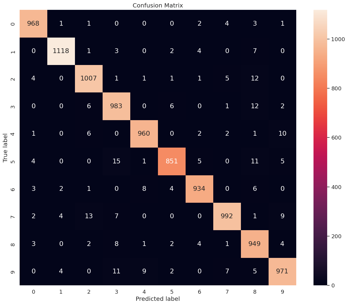
We obtain an accuracy score of \(0.9733\). Next, we compute and print the confusion matrix depicting the model performance on each class.
import pandas as pd
import seaborn as sns
from sklearn import metrics
def conf_mat(y_test, y_pred, num_class, figsize = (10, 8), font_scale = 1.2, annot_kws_size = 16):
    class_names = np.arange(num_class)
    tick_marks_y = np.arange(num_class) + 0.5
    tick_marks_x = np.arange(num_class) + 0.5
    confusion_matrix = metrics.confusion_matrix(y_test, y_pred)
    confusion_matrix_df = pd.DataFrame(confusion_matrix, range(num_class), range(num_class))
    plt.figure(figsize = figsize)
    sns.set(font_scale = font_scale) # label size
    plt.title("Confusion Matrix")
    sns.heatmap(confusion_matrix_df, annot = True, annot_kws = {"size": annot_kws_size}, fmt = 'd') # font size
    plt.yticks(tick_marks_y, class_names, rotation = 'vertical')
    plt.xticks(tick_marks_x, class_names, rotation = 'horizontal')
    plt.ylabel('True label')
    plt.xlabel('Predicted label')
    plt.grid(False)
    plt.show()

conf_mat(y_test, y_pred, num_class = 10, figsize = (15, 12), font_scale = 1.2, annot_kws_size = 16)
○ References
- Accuracy
- Accuracy score documentation
- Activation function
- Adam optimizer
- Binary cross-entropy
- Confusion matrix
- Dense layer
- EarlyStopping callback
- imshow function
- Keras datasets
- Keras losses
- Keras optimizers
- Learning rate
- LearningRateScheduler callback
- MNIST database
- MNIST digits classification dataset
- ModelCheckpoint callback
- Neural network
- One-hot
- Pyplot module
- Scikit-learn metrics
- Sequential model