Implementing Logistic Regression from Scratch
Many advanced libraries, such as scikit-learn, make it possible to carry out training and inference with a few lines of code. While it is very convenient for day-to-day practice, it does not give insight into the details of what really happens underneath when we run those codes. In this note, we implement a logistic regression model manually from scratch, without using any advanced library, to understand how it works in the context of binary classification.
○ Contents
- Introduction
- Logistic Function
- Log Loss
- Cost Function
- Gradient Descent
- Preprocessing
- Model Fitting
- Prediction and Evaluation
- Regularization
- Acknowledgements
- References
○ Introduction
Classification. In statistics and machine learning, classification refers to a type of supervised learning. For this task, training data with known class labels are given and is used to develop a classification rule for assigning new unlabeled data to one of the classes. A special case of the task is binary classification, which involves only two classes. Some examples:
- Classifying an email as
spamornon-spam - Classifying a tumor as
benignormalignant
The algorithms that sort unlabeled data into labeled classes are called classifiers. Loosely speaking, the sorting hat from Hogwarts can be thought of as a classifier that sorts incoming students into four distinct houses. In real life, some common classifiers are logistic regression, k-nearest neighbors, decision tree, random forest, support vector machine, naive Bayes, linear discriminant analysis, stochastic gradient descent, XGBoost, AdaBoost, and neural networks.
The purpose of the note. Many advanced libraries, such as scikit-learn, make it possible for us to train various models on labeled training data, and predict on unlabeled test data, with a few lines of code. While it is very convenient for day-to-day practice, it does not give insight into the details of what really happens underneath when we run those codes. In this note, we implement a logistic regression model manually from scratch, without using any advanced library, to understand how it works in the context of binary classification. The basic idea is to segment the computations into pieces, and write functions to compute each piece in a sequential manner, so that we can build a function on the basis of the previously defined functions. Wherever applicable, we have complemented a function which is constructed using for loops, with a much faster vectorized implementation of the same.
A problem from particle physics. We have chosen the particular problem posed in this competition. In particle physics, an event refers to the results just after a fundamental interaction takes place between subatomic particles, occurring in a very short time span, at a well-localized region of space. The problem is to classify an event produced in a particle accelerator as background or signal, based on relevant feature variables. A background event is explained by the existing theories and previous observations. A signal event, however, indicates a process that cannot be described by previous observations and leads to the potential discovery of a new particle. More on this problem is detailed in the introduction section of this notebook.
Data. The dataset, provided with the competition, has been built from official ATLAS full-detector simulation. The simulator has two parts. In the first, random proton-proton collisions are simulated based on the knowledge that we have accumulated on particle physics. It reproduces the random microscopic explosions resulting from the proton-proton collisions. In the second part, the resulting particles are tracked through a virtual model of the detector. The process yields simulated events with properties that mimic the statistical properties of the real events with additional information on what has happened during the collision, before particles are measured in the detector. Information on \(250000\)
events are included int he dataset. For each event, it has information on \(31\)
features (\(2\)
integer-type features and \(29\)
float-type features). Additionally, the dataset contains the object-type target variable labels and float-type variable weights. The target variable can take two possible values: \(b\)
(indicating a background event) and \(s\)
(indicating a signal event).
Synopsis of the data
- Number of observations: \(250000\)
- Number of columns: \(33\)
- Number of integer columns: \(2\)
- Number of float columns: \(30\)
- Number of object columns: \(1\)
- Number of duplicate observations: \(0\)
- Constant columns: None
- Number of columns with missing values: \(0\)
- Memory Usage: \(62.94\) MB
○ Logistic Function
A function \(g: \mathbb{R} \to \mathbb{R}\) is said to be a sigmoid function if it has the following properties:
- It is bounded.
- It is differentiable.
- It has nonnegative derivative at each point.
- It has exactly one inflection point.
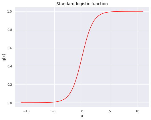
An example of a sigmoid function is the standard logistic function (sometimes simply referred to as the sigmoid), which is given by
for \(x \in \mathbb{R}\). The next code block constructs this function.
def logistic(x):
    """
    Computes the logistic function applied to an input scalar/array
    Args:
        x (scalar/ndarray): scalar or numpy array of any size
    Returns:
        y (scalar/ndarray): logistic function applied to x, has the same shape as x
    """
    y = 1 / (1 + np.exp(-x))
    return y
○ Log Loss
The loss function, which corresponds to the true value and predicted value of a single observation. The cost function can be thought of as expected loss or average loss over a group of observations. Contrary to linear regression, which employs squared loss, logistic regression makes use of the log loss function, given by
where \(y\) is the true value of a binary target (taking values \(0\) or \(1\)) and \(y'\) is the prediction, which can be thought of as the predicted probability of \(y\) being \(1\).
Observe that the loss is \(0\), when the true value and predicted value agree with each other, i.e., \(L(0, 0) = L(1, 1) = 0\).
On the other hand, the loss explodes towards infinity if the predicted value approaches \(1\) when the true value is \(0\), or it approaches \(0\) when the true value is \(1\). Mathematically,
Next, we construct the function to compute log loss and plot it for \(y = 0\) and \(y = 1\). Since the true values (labels) are always \(0\) or \(1\), we do not need to pay heed to the behaviour of the function \(L\) for other values of \(y\).
def log_loss(y, y_dash):
    """
    Computes log loss for inputs true value (0 or 1) and predicted value (between 0 and 1)
    Args:
      y      (scalar): true value (0 or 1)
      y_dash (scalar): predicted value (probability of y being 1)
    Returns:
      loss (float): nonnegative loss corresponding to y and y_dash
    """
    loss = - (y * np.log(y_dash)) - ((1 - y) * np.log(1 - y_dash))
    return loss
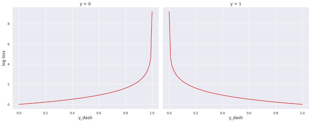
The plots sync with the intuition that loss should be minimum when the predicted value (probability) matches the true value (\(0\) or \(1\)) and should increase as the two values drift apart.
○ Cost Function
Let \(\mathbf{y} = (y_1, y_2, \cdots, y_n)\) be the true values (\(0\) or \(1\)) and \(\mathbf{y'} = (y_1', y_2', \cdots, y_n')\) be the corresponding predictions (probabilities). Then, the cost function is given by the average loss:
We construct the function to compute cost. An important structural distinction from the log loss function is that here the arguments y and y_dash are vectors, not scalars.
def cost_func(y, y_dash):
    """
    Computes log loss for inputs true value (0 or 1) and predicted value (between 0 and 1)
    Args:
      y      (array_like, shape (m,)): array of true values (0 or 1)
      y_dash (array_like, shape (m,)): array of predicted values (probability of y being 1)
    Returns:
      cost (float): nonnegative cost corresponding to y and y_dash
    """
    assert len(y) == len(y_dash), "Length of true values and length of predicted values do not match"
    m = len(y)
    cost = 0
    for i in range(m):
        cost += log_loss(y[i], y_dash[i])
    cost = cost / m
    return cost
The previous function computes cost using for loop. Now, we compute the same using vectorization.
def cost_func_vec(y, y_dash):
    """
    Computes log loss for inputs true value (0 or 1) and predicted value (between 0 and 1)
    Args:
      y      (array_like, shape (m,)): array of true values (0 or 1)
      y_dash (array_like, shape (m,)): array of predicted values (probability of y being 1)
    Returns:
      cost (float): nonnegative cost corresponding to y and y_dash
    """
    assert len(y) == len(y_dash), "Length of true values and length of predicted values do not match"
    m = len(y)
    loss_vec = np.array([log_loss(y[i], y_dash[i]) for i in range(m)])
    cost = np.dot(loss_vec, np.ones(m)) / m
    return cost
Let us assume that we want to predict \(y\) based on \(n\) features. In this setup, a logistic regression model is characterized by \(n+1\) parameters:
- weight parameters \(\mathbf{w} = (w_1, w_2, \cdots, w_n)\)
- bias parameter \(b\)
Note that, the dot product of two vectors \(\mathbf{a} = (a_1, a_2, \cdots, a_n)\) and \(\mathbf{b} = (b_1, b_2, \cdots, b_n)\) is given by \(\mathbf{a} \cdot \mathbf{b} = \sum_{i=1}^n a_ib_i\). It is a scalar value and evidently, \(\mathbf{a} \cdot \mathbf{b} = \mathbf{b} \cdot \mathbf{a}\). Given the realized values of \(n\) features \(\mathbf{x} = (x_1, x_2, \cdots, x_n)\), the model feeds \(\mathbf{x} \cdot \mathbf{w} + b\) to the logistic function \(g\), and projects the output as the predicted probability of \(y = 1\). Concretely, we have
Let us consider the situation of \(m\) observations, with the \(i\)th observation having feature values \(\mathbf{x_i} = (x_{i,1}, x_{i,2}, \cdots, x_{i,n})\), true target value \(y_i\) and predicted probabilities \(y_i' = g\left(\mathbf{x_i} \cdot \mathbf{w} + b\right)\). Stacking them up, we obtain the feature matrix \(\mathbf{X}\), target vector \(\mathbf{y}\) and the vector of predicted probability \(\mathbf{y'}\), as follows:
Now, we are in a position to rewrite the cost function in terms of model parameters:
Note that \(J\left(\mathbf{0}, 0\right) = \log{2}\) for every input data \(\mathbf{X}\) (features) and \(\mathbf{y}\) (target). We construct a function to compute the cost, given data and model parameters, in the general setup of \(n\) features.
def cost_logreg(X, y, w, b):
    """
    Computes the cost function, given data and model parameters
    Args:
      X (ndarray, shape (m,n))  : data on features, m observations with n features
      y (array_like, shape (m,)): array of true values (0 or 1) of target
      w (array_like, shape (n,)): weight parameters of the model
      b (float)                 : bias parameter of the model
    Returns:
      cost (float): nonnegative cost corresponding to y and y_dash
    """
    m, n = X.shape
    assert len(y) == m, "Number of feature observations and number of target observations do not match"
    assert len(w) == n, "Number of features and number of weight parameters do not match"
    z = []
    for i in range(m):
        s = 0
        for j in range(n):
            s += X[i, j] * w[j]
        z.append(s + b)
    z = np.array(z)
    y_dash = logistic(z)
    cost = cost_func(y, y_dash)
    return cost
The code for logistic function \(g\) is constructed in such a way that, if applied on an array, it acts separately on each component and returns an array. Using this, it follows from \((2)\) that
where \(\mathbf{1}\) has the same dimension as that of \(\mathbf{X} \mathbf{w}\). We use matrix multiplication in computing \(\mathbf{X} \mathbf{w}\), scalar multiplication of a vector in computing \(b \mathbf{1}\) and add them up using vector addition. This representation leads to a much faster vectorized implementation of computing the cost function in terms of model parameters.
def cost_logreg_vec(X, y, w, b):
    """
    Computes the cost function, given data and model parameters
    Args:
      X (ndarray, shape (m,n))  : data on features, m observations with n features
      y (array_like, shape (m,)): array of true values of target (0 or 1)
      w (array_like, shape (n,)): weight parameters of the model
      b (float)                 : bias parameter of the model
    Returns:
      cost (float): nonnegative cost corresponding to y and y_dash
    """
    m, n = X.shape
    assert len(y) == m, "Number of feature observations and number of target observations do not match"
    assert len(w) == n, "Number of features and number of weight parameters do not match"
    z = np.matmul(X, w) + (b * np.ones(m))
    y_dash = logistic(z)
    cost = cost_func_vec(y, y_dash)
    return cost
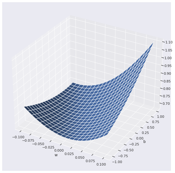
We visualize the cost function for a simplified setup, consisting of a single feature \(x\). In this setup, the model involves two parameters only, the weight parameter \(w\) and the bias parameter \(b\).
The prediction \(y'\) in \((1)\) can be converted to a decision by using a threshold value. For instance, suppose we take the threshold to be \(0.5\). Then, we may classify the observation to class \(1\) if \(y' \geq 0.5\), and to class \(0\) otherwise. The problem, however, is that we do not know the model parameters \(\mathbf{w}\) and \(b\), and hence cannot compute \(y'\) directly. First, we have to fit the model by finding the best fitting parameters. Observe that, given the training data, \(C\left(\mathbf{y}, \mathbf{y'}\right)\) depends on \(\mathbf{w}\) and \(b\) only. A reasonable strategy, therefore, is:
We shall employ the gradient descent algorithm to solve this optimization problem.
○ Gradient Descent
What is it? The gradient descent algorithm is a first order iterative optimization algorithm for finding a local minimum of a differentiable function. The idea is to take repeated steps in the opposite direction of the gradient (or approximate gradient) of the function at the current point, because this is the direction of steepest descent. Conversely, stepping in the direction of the gradient will lead to a local maximum of that function. This procedure is then known as gradient ascent.
History. Gradient descent is generally attributed to Augustin-Louis Cauchy, who first suggested it in \(1847\). Jacques Hadamard independently proposed a similar method in \(1907\). Its convergence properties for non-linear optimization problems were first studied by Haskell Curry in \(1944\), with the method becoming increasingly well-studied and used in the following decades.
The algorithm. In the context of minimising the cost function \(J\), with respect to the model parameters \(\mathbf{w}\) and \(b\), the gradient descent algorithm is given by:
where \(\alpha\) is the learning rate, and the parameters \(\mathbf{w} = (w_1, w_2, \cdots, w_n)\) and \(b\) are updated simultaniously in each iteration.
Computing gradient. Before we can implement the gradient descent algorithm, we need to compute the gradients first. From \((3)\), we can compute the partial derivatives of \(J\) with respect to \(w_j\) and \(b\) as follows:
Next, we construct a function to compute these gradients.
def grad_logreg(X, y, w, b):
    """
    Computes gradients of the cost function with respect to model parameters
    Args:
      X (ndarray, shape (m,n))  : data on features, m observations with n features
      y (array_like, shape (m,)): array of true values of target (0 or 1)
      w (array_like, shape (n,)): weight parameters of the model
      b (float)                 : bias parameter of the model
    Returns:
      grad_w (array_like, shape (n,)): gradients of the cost function with respect to the weight parameters
      grad_b (float)                 : gradient of the cost function with respect to the bias parameter
    """
    m, n = X.shape
    assert len(y) == m, "Number of feature observations and number of target observations do not match"
    assert len(w) == n, "Number of features and number of weight parameters do not match"
    grad_w, grad_b = np.zeros(n), 0
    for i in range(m):
        s = 0
        for j in range(n):
            s += X[i, j] * w[j]
        y_dash_i = logistic(s + b)
        for j in range(n):
            grad_w[j] += (y_dash_i  - y[i]) * X[i,j]
        grad_b += y_dash_i  - y[i]
    grad_w, grad_b = grad_w / m, grad_b / m
    return grad_w, grad_b
The next function computes the same using vectorization.
def grad_logreg_vec(X, y, w, b):
    """
    Computes gradients of the cost function with respect to model parameters
    Args:
      X (ndarray, shape (m,n))  : data on features, m observations with n features
      y (array_like, shape (m,)): array of true values of target (0 or 1)
      w (array_like, shape (n,)): weight parameters of the model
      b (float)                 : bias parameter of the model
    Returns:
      grad_w (array_like, shape (n,)): gradients of the cost function with respect to the weight parameters
      grad_b (float)                 : gradient of the cost function with respect to the bias parameter
    """
    m, n = X.shape
    assert len(y) == m, "Number of feature observations and number of target observations do not match"
    assert len(w) == n, "Number of features and number of weight parameters do not match"
    y_dash = logistic(np.matmul(X, w) + b * np.ones(m))
    grad_w = np.matmul(y_dash - y, X) / m
    grad_b = np.dot(y_dash - y, np.ones(m)) / m
    return grad_w, grad_b
Armed with the required functions, we can now implement the gradient descent algorithm, given in \((4)\).
def grad_desc(X, y, w, b, alpha, n_iter, show_cost = True, show_params = False):
    """
    Implements batch gradient descent algorithm to learn and update model parameters
    with prespecified number of interations and learning rate
    Args:
      X (ndarray, shape (m,n))  : data on features, m observations with n features
      y (array_like, shape (m,)): true values of target (0 or 1)
      w (array_like, shape (n,)): initial value of weight parameters
      b (scalar)                : initial value of bias parameter
      alpha (float)             : learning rate
      n_iter (int)              : number of iterations
      show_cost (Boolean)       : if true, prints the cost associated with some iterations
      show_params (Boolean)     : if true, additionally prints the corresponding parameter values (effective only if show_cost is true)
    Returns:
      w (array_like, shape (n,))                       : updated values of weight parameters
      b (scalar)                                       : updated value of bias parameter
      cost_history (array_like, shape (len(n_iter),))  : list of cost values associated with each iteration
      params_history (array_like, shape (len(n_iter),)): list of parameter values associated with each iteration
    """
    m, n = X.shape
    assert len(y) == m, "Number of feature observations and number of target observations do not match"
    assert len(w) == n, "Number of features and number of weight parameters do not match"
    cost_history, params_history = [], []
    for i in range(n_iter):
        grad_w, grad_b = grad_logreg_vec(X, y, w, b)
        w += - alpha * grad_w
        b += - alpha * grad_b
        cost =  cost_logreg_vec(X, y, w, b)
        cost_history.append(cost)
        params_history.append([w, b])
        if show_cost == True and show_params == False and (i % math.ceil(n_iter / 10) == 0 or i == n_iter - 1):
            print(f"Iteration {i:6}:    Cost  {float(cost_history[i]):3.4f}")
        if show_cost == True and show_params == True and (i % math.ceil(n_iter / 10) == 0 or i == n_iter - 1):
            print(f"Iteration {i:6}:    Cost  {float(cost_history[i]):3.4f},    Params  {params_history[i]}")
    return w, b, cost_history, params_history
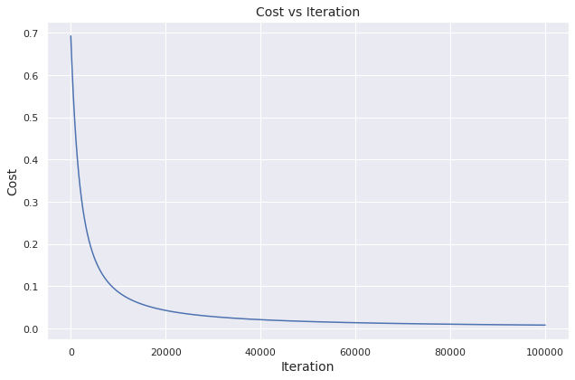
To demonstrate, we take example inputs and feed them to the function. If implemented properly, the cost should diminish over iterations.
X, y = np.array([[0.1, 0.2], [-0.1, 0.1]]), np.array([1, 0])
w, b, alpha, n_iter = np.array([0., 0.]), 0., 0.1, 100000
w_out, b_out, cost_history, params_history = grad_desc(X, y, w, b, alpha, n_iter, show_cost = True, show_params = True)

We visualize how the cost evolves over iterations.
○ Preprocessing
The columns EventId and Weight will not be used in this notebook. Thus we drop these columns.
data.drop(['EventId', 'Weight'], axis = 1, inplace = True)
Even though there are no NaN values in the dataset, we observe that several columns unnaturally contain the value \(-999\)
for many observations. We suspect that these are missing or corrupted values that have been replaced with \(-999\)
and we convert them to np.nan. We shall impute these values after train-test split.
data.replace(to_replace = -999, value = np.nan, inplace = True)
Furthermore, we encode the Label column as follows: \(b \mapsto 0\)
and \(s \mapsto 1\).
label_dict = {'b': 0, 's': 1}
data.replace({'Label': label_dict}, inplace = True)
Next, we split data into two parts:
data_train: The portion of data that we use to train the modelsdata_test: The portion of data that we use to test or evaluate the models
data_train, data_test = train_test_split(data, test_size = 0.2, random_state = 40)
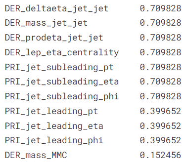
Next, we identify \(11\)
columns with missing values. Among them, \(10\)
columns have more than \(30\%\)
data missing, and hence we shall discard them. The column DER_mass_MMC has about \(15.25\%\)
data missing. We show the relative frequency of missing values in these columns.
(data.isna().sum()[data.isna().sum() > 0] / len(data)).sort_values(ascending = False)
cols_missing_drop = data.isna().sum()[data.isna().sum() / len(data) > 0.3].index.tolist()
data_train.drop(cols_missing_drop, axis = 1, inplace = True)
data_test.drop(cols_missing_drop, axis = 1, inplace = True)
We impute the missing values in the DER_mass_MMC column by the median of the rest of the values in the column.
data_train['DER_mass_MMC'].fillna(data_train['DER_mass_MMC'].median(), inplace = True)
data_test['DER_mass_MMC'].fillna(data_test['DER_mass_MMC'].median(), inplace = True)
Next, we shall split the data into features and target.
def predictor_target_split(data, target):
    X = data.drop(target, axis = 1)
    y = data[target]
    return X, y
X_train, y_train = predictor_target_split(data_train, 'Label')
X_train, y_train = predictor_target_split(data_train, 'Label')
We normalize the data, so that each column has values in the similar scale.
from sklearn.preprocessing import MinMaxScaler
def scaler(X_train, X_test):
    scaling = MinMaxScaler().fit(X_train)
    X_train_scaled = scaling.transform(X_train)
    X_test_scaled = scaling.transform(X_test)
    return X_train_scaled, X_test_scaled
X_train, X_test = scaler(X_train, X_test)
○ Model Fitting
We fix the initial values of the parameters, based on running the algorithm several times and noting down the final parameter values. It gives us a better starting point and helps to achieve a better performance in a limited number of iterations.
w_init = np.array([-5, -15, -10, 9, 4, -6, 3, -10, 1, 14, 0, 0, 15, 0, 0, 7, 0, -3, 1, -8]).astype(float)
b_init = -1.
Next, we learn the model parameters using gradient descent algorithm.
w_out, b_out, cost_history, params_history = grad_desc(
    X_train.to_numpy(),
    y_train.to_numpy(),
    w = w_init, # np.zeros(X_train.shape[1]),
    b = b_init, # 0,
    alpha = 0.1,
    n_iter = 2000,
    show_cost = True,
    show_params = False
)
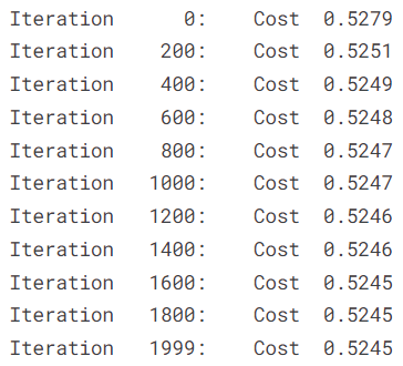
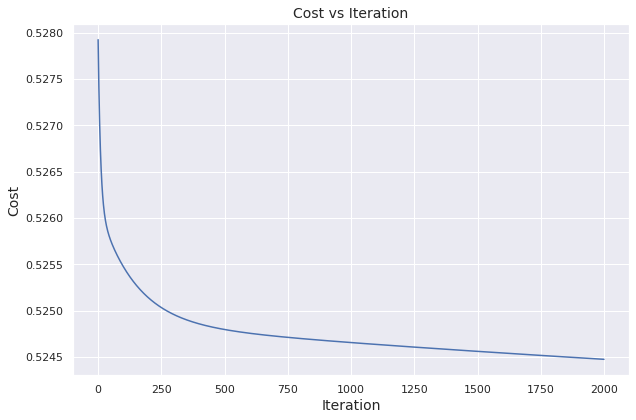
We visualize how the cost evolves over iterations.
The final values of the parameters \(\mathbf{w}\)
and \(b\),
stored in w_out and b_out, respectively, are given below.

○ Prediction and Evaluation
We use the final parameter values w_out and b_out to predict the positive class probabilities for both the training observations and the test observations.
y_train_prob = logistic(np.matmul(X_train.to_numpy(), w_out) + (b_out * np.ones(X_train.shape[0])))
y_test_prob = logistic(np.matmul(X_test.to_numpy(), w_out) + (b_out * np.ones(X_test.shape[0])))
Now, we convert the predicted class probabilities to class labels.
y_train_pred = (y_train_prob > 0.5).astype(int)
y_test_pred = (y_test_prob > 0.5).astype(int)
We evaluate the model performance on the training set and the test set through the accuracy metric.

The confusion matrix, depicting the test set performance, is given below.

○ Regularization
Regularization provides a tool to deal with overfitting. Essentially it puts a restriction the parameter values by adding a term in the cost function. This way, it prevents the model from fitting too well on the training set and failing to generalize on the test set. The following is one way to do this:
where \(\lambda \geq 0\) is called the regularization parameter.
Evidently, if \(\lambda = 0\), we get back the previous setup. Thus, the new cost function, parameterized by \(\lambda\), gives a generalization of the setup described in the previous sections.
The setup in \((5)\) is called the \(L_2\) regularization, as the regularization term essentially is \((\lambda/2m)\,\Vert \mathbf{w} \Vert_2^2\), i.e., the \(l^2\) norm of \(\mathbf{w}\), multiplied by the term \((\lambda/2m)\).
In this section, we shall employ the \(L_2\) regularization on the cost function, given in \((3)\), and check if it improves performance of the logistic regression model, derived thence. We rewrite the functions to compute cost, gradient and to implement gradient descent algorithm, incorporating regularization with the extra parameter \(l\).
We begin with the function to compute regularized cost function in terms of model parameters using for loops.
def cost_logreg_reg(X, y, w, b, l):
    """
    Computes the cost function, given data and model parameters
    Args:
      X (ndarray, shape (m,n))  : data on features, m observations with n features
      y (array_like, shape (m,)): array of true values (0 or 1) of target
      w (array_like, shape (n,)): weight parameters of the model
      b (float)                 : bias parameter of the model
      l (float)                 : regularization parameter
    Returns:
      cost (float): nonnegative cost corresponding to y and y_dash
    """
    m, n = X.shape
    assert len(y) == m, "Number of feature observations and number of target observations do not match"
    assert len(w) == n, "Number of features and number of weight parameters do not match"
    cost = cost_logreg(X, y, w, b)
    for j in range(n):
        cost += (l / (2 * m)) * (w[j]**2)
    return cost
Next, we implement the same using vectorization.
def cost_logreg_vec_reg(X, y, w, b, l):
    """
    Computes the cost function, given data and model parameters
    Args:
      X (ndarray, shape (m,n))  : data on features, m observations with n features
      y (array_like, shape (m,)): array of true values (0 or 1) of target
      w (array_like, shape (n,)): weight parameters of the model
      b (float)                 : bias parameter of the model
      l (float)                 : regularization parameter
    Returns:
      cost (float): nonnegative cost corresponding to y and y_dash
    """
    m, n = X.shape
    assert len(y) == m, "Number of feature observations and number of target observations do not match"
    assert len(w) == n, "Number of features and number of weight parameters do not match"
    cost = cost_logreg_vec(X, y, w, b)
    cost += (l / (2 * m)) * np.dot(w, w)
    return cost
From \((5)\), we can compute the modified partial derivatives of \(J\) with respect to \(w_j\) and \(b\) as follows:
We construct a function to compute these gradients using for loops.
def grad_logreg_reg(X, y, w, b, l):
    """
    Computes gradients of the cost function with respect to model parameters
    Args:
      X (ndarray, shape (m,n))  : data on features, m observations with n features
      y (array_like, shape (m,)): array of true values of target (0 or 1)
      w (array_like, shape (n,)): weight parameters of the model
      b (float)                 : bias parameter of the model
      l (float)                 : regularization parameter
    Returns:
      grad_w (array_like, shape (n,)): gradients of the cost function with respect to the weight parameters
      grad_b (float)                 : gradient of the cost function with respect to the bias parameter
    """
    m, n = X.shape
    assert len(y) == m, "Number of feature observations and number of target observations do not match"
    assert len(w) == n, "Number of features and number of weight parameters do not match"
    grad_w, grad_b = grad_logreg(X, y, w, b)
    for j in range(n):
        grad_w[j] += (l / m) * w[j]
    return grad_w, grad_b
Next, we implement the same using vectorization.
def grad_logreg_vec_reg(X, y, w, b, l):
    """
    Computes gradients of the cost function with respect to model parameters
    Args:
      X (ndarray, shape (m,n))  : data on features, m observations with n features
      y (array_like, shape (m,)): array of true values of target (0 or 1)
      w (array_like, shape (n,)): weight parameters of the model
      b (float)                 : bias parameter of the model
      l (float)                 : regularization parameter
    Returns:
      grad_w (array_like, shape (n,)): gradients of the cost function with respect to the weight parameters
      grad_b (float)                 : gradient of the cost function with respect to the bias parameter
    """
    m, n = X.shape
    assert len(y) == m, "Number of feature observations and number of target observations do not match"
    assert len(w) == n, "Number of features and number of weight parameters do not match"
    grad_w, grad_b = grad_logreg_vec(X, y, w, b)
    grad_w += (l / m) * w
    return grad_w, grad_b
Using the regularised cost function and its gradients with respect to the model parameters, we construct a function to implement the gradient descent algorithm for logistic regression, incorporating regularization. Specifically, the algorithm learns the model parameters, with the goal of minimizing the regularised cost function in \((5)\), instead of the usual cost function in \((3)\).
def grad_desc_reg(X, y, w, b, l, alpha, n_iter, show_cost = True, show_params = False):
    """
    Implements batch gradient descent algorithm to learn and update model parameters
    with prespecified number of interations and learning rate
    Args:
      X (ndarray, shape (m,n))  : data on features, m observations with n features
      y (array_like, shape (m,)): true values of target (0 or 1)
      w (array_like, shape (n,)): initial value of weight parameters
      b (scalar)                : initial value of bias parameter
      l (float)                 : regularization parameter
      alpha (float)             : learning rate
      n_iter (int)              : number of iterations
      show_cost (Boolean)       : if true, prints the cost associated with some iterations
      show_params (Boolean)     : if true, additionally prints the corresponding parameter values (effective only if show_cost is true)
    Returns:
      w (array_like, shape (n,))                       : updated values of weight parameters
      b (scalar)                                       : updated value of bias parameter
      cost_history (array_like, shape (len(n_iter),))  : list of cost values associated with each iteration
      params_history (array_like, shape (len(n_iter),)): list of parameter values associated with each iteration
    """
    m, n = X.shape
    assert len(y) == m, "Number of feature observations and number of target observations do not match"
    assert len(w) == n, "Number of features and number of weight parameters do not match"
    cost_history, params_history = [], []
    for i, j in itertools.product(range(n_iter), range(1)):
        grad_w, grad_b = grad_logreg_vec_reg(X, y, w, b, l)
        w += - alpha * grad_w
        b += - alpha * grad_b
        cost =  cost_logreg_vec_reg(X, y, w, b, l)
        cost_history.append(cost)
        params_history.append([w, b])
        if show_cost == True and show_params == False and (i % math.ceil(n_iter / 10) == 0 or i == n_iter - 1):
            print(f"Iteration {i:6}:    Cost  {float(cost_history[i]):3.4f}")
        if show_cost == True and show_params == True and (i % math.ceil(n_iter / 10) == 0 or i == n_iter - 1):
            print(f"Iteration {i:6}:    Cost  {float(cost_history[i]):3.4f},    Params  {params_history[i]}")
    return w, b, cost_history, params_history
We use the same initial values for the model parameters as in the unregularized implementation.
w_init = np.array([-5, -15, -10, 9, 4, -6, 3, -10, 1, 14, 0, 0, 15, 0, 0, 7, 0, -3, 1, -8]).astype(float)
b_init = -1.
Next, we learn the model parameters using gradient descent algorithm.
w_out_reg, b_out_reg, cost_history_reg, params_history_reg = grad_desc_reg(
    X_train.to_numpy(),
    y_train.to_numpy(),
    w = w_init, # np.zeros(X_train.shape[1]),
    b = b_init, # 0,
    l = 1.,
    alpha = 0.1,
    n_iter = 2000
)
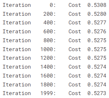
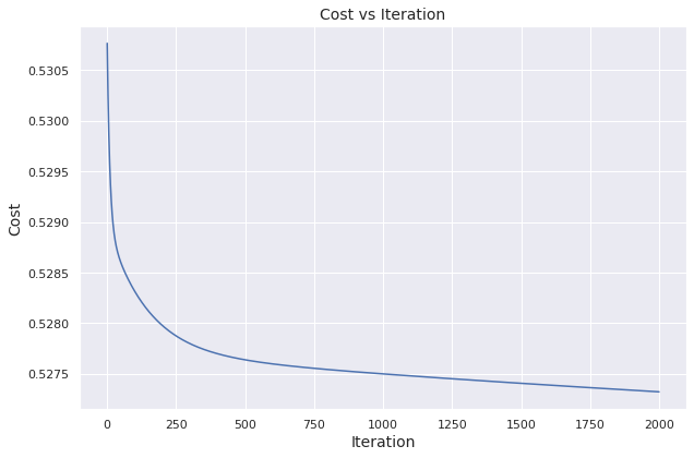
We visualize how the cost evolves over iterations.
The final values of the parameters \(\mathbf{w}\)
and \(b\),
stored in w_out_reg and b_out_reg, respectively, are given below.

We use the final parameter values w_out_reg and b_out_reg to predict the positive class probabilities for both the training observations and the test observations.
y_train_prob_reg = logistic(np.matmul(X_train.to_numpy(), w_out_reg) + (b_out_reg * np.ones(X_train.shape[0])))
y_test_prob_reg = logistic(np.matmul(X_test.to_numpy(), w_out_reg) + (b_out_reg * np.ones(X_test.shape[0])))
Now, we convert the predicted class probabilities to class labels.
y_train_pred_reg = (y_train_prob_reg > 0.5).astype(int)
y_test_pred_reg = (y_test_prob_reg > 0.5).astype(int)
We evaluate the model performance on the training set and the test set through the accuracy metric.

The confusion matrix, depicting the test set performance, is given below.
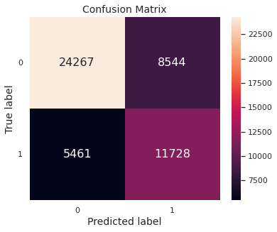
Thus, in this scenario, regularization does not help much. This is expected since the unregularized implementation does not indicate overfitting.
○ Acknowledgements
○ References
- Accuracy
- AdaBoost
- Algorithm
- Augustin-Louis Cauchy
- Binary classification
- Bounded function
- Classification rule
- Confusion matrix
- Decision tree
- Differentiable function
- Dot product
- First order methods
- Fundamental interaction
- Gradient
- Gradient descent
- Haskell Curry
- Hogwarts
- Inflection point
- Jacques Hadamard
- K-nearest neighbors algorithm
- \(l^2\) norm
- Learning rate
- Linear discriminant analysis
- Logistic function
- Logistic regression
- Machine learning
- Matrix multiplication
- Maxima and minima
- Naive Bayes classifier
- Neural network
- Optimization
- Particle physics
- Random forest
- Regularization
- Scalar multiplication
- Scikit-learn
- Sigmoid function
- Sorting hat
- Statistical classification
- Statistics
- Stochastic gradient descent
- Subatomic particle
- Supervised learning
- Support vector machine
- Test data
- Training data
- Vector addition
- XGBoost